Category Archives: surfactant proteins A and D

Sub-peaks found within the “reasonably well documented” 8 peaks per SP-D trimer

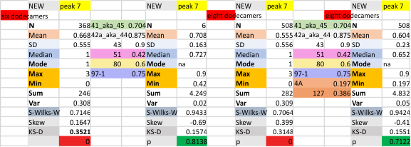
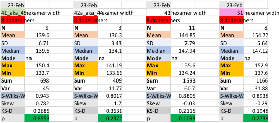
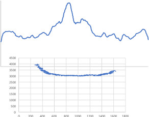
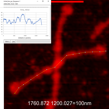
These data show the number of smaller peaks within the tracings of SP-D trimers (using AFM images from various published papers). At this point they are all rhSP-D images. The trimers are plotted beginning at the most complete side of the N term peak. This means that the whole N term is plotted (and it includes the N from the adjacent trimer(s) that build a dodecamer. All these plots are from dodecamers. This link is to a summary of the number of sub-peaks.
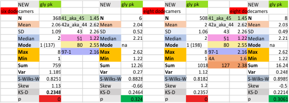
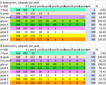
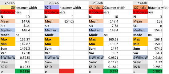
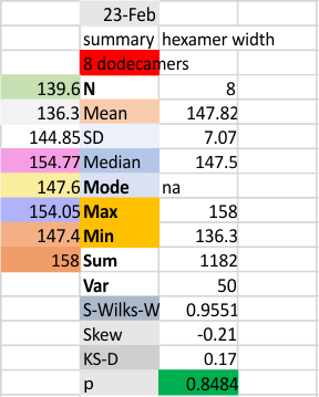
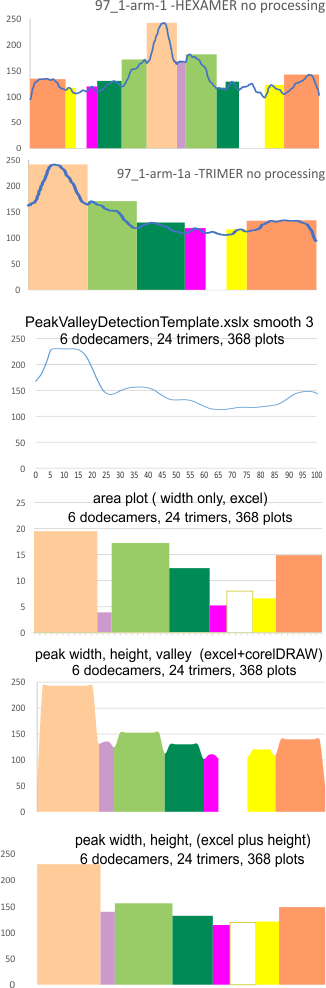
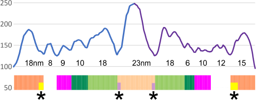
It has been my observation that the multimers of SP-D with higher than four trimer arms often show a decreased brightness within the center, and many images confirm this. In this series of plots there are just a few images where in a plot of a hexamer, there is a small peak in the center of the N term peak. I have labeled it the ? peak, and it is shown below in light bluegreen.  It doesn’t occur often but enough to mention it. All the data are organized similarly. On the far left is the sum total of peaks from six hexamers (n of trimers =368 which includes gray  scale plots from many signal and image processed images, so on the very left, no division into dodecamers is made, but the column just to the right of that has six dodecamers where the mean occurrence of peaks is found where the N=6.  On the right hand side of the data, far right, the same has been applied to 8 dodecamers, and just to the left of that set of numbers is data for each individual trimer, and n=508 plots.
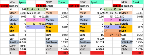
While signal processing apps have determined that there are likely 15 peaks per hexamer, this number does NOT include the ? peak above.

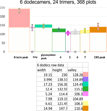
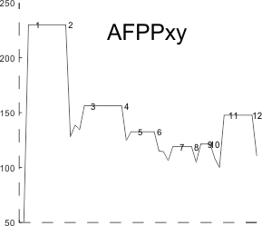
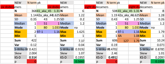
The 8 peaks per trimer (N peak is counted once with each trimer, but also counted only once with each hexamer) are as follows:

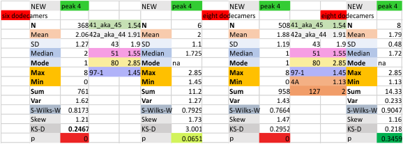
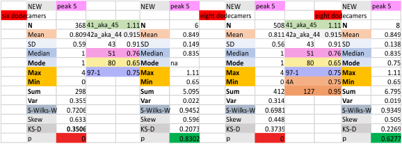
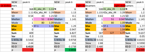
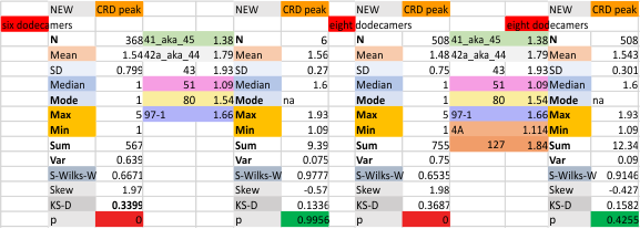
N term peak, tiny unidentified peak, glycosylation peak, peak 4, peak 5, peak 6, coiled neck peak 7, CRD peak 8, and are labeled like this below. The means are the number of sub-peaks per peak.  The three confirmed peaks (in the literature are N, gly and CRD, the neck peak 7 is inconsistent because the CRD domains obstruct it often. Peaks that are NEW, and as yet unconfirmed are tiny peak (2), peak 4, 5, and 6).

The N term peak has been organized with the mean of the sub-peaks per N term peak plotted from the same trimers as above. And so on, for each of the peaks — as listed above.


The glycosylation peak is apt to be not just one peak but two (and my thought is because each of the trimers can by glycosylated individually, and the coil of the trimer ofsets each of those sub-peaks.  Those peaks composed of more than one sub-peak are the glycosylation peak (peak 2) and an as yet undescribed peak 4 which also has two sub-peaks.  The CRD domain is subject to a different type of flopping around, and does not show two peaks consistently. This is likely affected by the fact that a plot line goes through the CRD often not picking up the apparently random order that the CRD domains of the trimer fall during processing.


8 dodecamersL SP-D: Subpeaks per peaks detected using AFM images of surfactant protein D.

8 dodecamersL SP-D: Subpeaks per peaks detected using AFM images of surfactant protein D. (APOLOGETICS) Always and at the outset I thank Arroyo et al for the 2020, 2018 publication of the SP-D AFM images (the best I have encountered of SP-D), and secondly I thank Dan Miller for the scipy app for peak finding, Aaron Miller for the LTI app for peak finding and batch processing, and Thomas O’Haver for his help with Octave, and excel templates, and also for ImageJ and Gwyddion (and I guess i should be very grateful for the original developers of CorelDRAW (which was Kodak)(not the new owners as they get a thumbs down from me), and also the original producers of Photoshop (yep, version 6 on CDs performed just as well for image analysis as rented versions of 2021 (so it is also thumbs down to them)).

The following is the result of 508 image and signal processing plots of 8 images of surfactant protein D. These data are reported as individual plots of hexamers (thus four trimer plots (as separate entities, with plots beginning at the full width of the N term plot and progressing to the CRD.  I have made the assumption (which I will discuss) that signal processing algorithms are smart enough to see symmetry… bilateral symmetry, which apparently is giving that AI too much credit.

Notwithstanding that problem, the total number of peaks per trimer (8) established some time ago is the number which is used to box the number of subpeaks into 8. Below are the data for 6 dodecamers (n = number of plots analyzed, not the number of dodecamers analyzed) and 8 dodecamers. Consistency is apparent. Not all peaks show up 100% of the time. Peaks such as the N and glycosylation and peak 5 and CRD peaks are often lumpy (meaning they have subpeaks.

There is a peak called “?” which only rarely occurs in dodecamers (but in my opinion is frequent in multimers (called fuzzy balls) and is indicative of a side to side N term association among molecules. It is reasonable for that peak NOT to show up below.

The N peak is present 100% of the time, as is the CRD peak and the glycosylation peak (though the height of the glycos peak varies (and at this point unglycosylated AFM images of SP-D have not been analyzed, so that will be dependent on the SP-D molecule, which species, and mutations and other factors, but here it is rhSP-D). Peak 4 is very consistent, present 99+ percent of the time, not previously reported, lying in the collagen-like domain. The next two peaks have characteristics that are obvious visually, peak 5 is not wide, and is not tall but consistently shows up right after peak 5. Peak 6 is broad, and appears regularly (94+ percent of the time, and is also low.  Peak 7 is what I believe is the neck of the SP-D trimer, and it is very often covered by the bright peak of the CRD (and this depends on whether the rounded ball shaped CRD peaks are positioned directly over the neck or to one side.  (Just my opinion here).  The glycosylation peak and peak typically have more than one subpeak.

8 dodecamers of SP-D

Two sets of measurements have been added to the dataset for hexamer (that would be the CRD to CRD measurement of two trimers with N terms meeting in the center of the dodecamer) (Numbers of the molecules are my assignments  (out of about 90 different images) and number 127, and figure 4A,  are both images of the same molecule, but found in separate figures from Arroyo et al). Different image processing apps have been applied to strengthen the signal from the peaks from all images, and each image then was subjected to signal processing peak findings (5 different apps and settings which are now used for on all plots of images).

The data for hexamer width have really changed from previous analyses, i dont think more will be useful in determining the hexamer width.  I will still do this (just to find outliers and potential mistakes) in the upcoming images that I analyze.

Early data is on this blog….  you can check if you like.

Feb 23 data with 8 molecules processed in almost 900 different plots is summarized below.  The diameter and the length of the arms is calculated separately (in nm, relying on the nm bar markers in each image used).  THe total number of times the hexamers are measured is less than the total number of times the trimer widths are plotted since the same image is used for the signal processing (thus repeating it, while it makes very little difference in the statistics) has not been done here.

6 dodecamers, 368 trimer plots, peak width, height, valley plots

EDIT: the plot shown below is what I think describes the data. It has the mean peak height, peak width and peak valley from 6 molecules. No smoothing or blur or anything else, just the numbers. It might be as useful as anything that some algorithm can invent.  Peak width is x, mean for the six molecules (the number of peaks per trimer and hexamer was determined by signal and image processing data early on) (15) and per trimer ( 8) respectively.

Number of peaks from each program depended upon various parameters, lag, threshold, influence, smoothing, and many I dont understand, but the separation of the signal and image processing graphs into the 8 peaks (color coded) was was performed by me, which, in my humble opinion, is just as good, if not more “learned” than any AI app.

The separation of each hexamer (or trimer) into peaks is reasonably consistent in terms of peak width, height and valleys.  THus I have means for all tracings, means for individual molecules, plus SD for widths, heights, and valleys, all of which can be given in table form shown below.

Means of all plots, and individual trimers dodecamers can be shown in the style of graph below, with SD of each parameter. The top image here is just a quick graphic of what that kind of plot would look like,  and are close to the actual numbers below but not exact, as this is a draft.  Peak width is in nm, peak height and valley are in grayscale 0-255.

Anyway, it is the format that I will use for collecting data on the remainder of the SP-D molecules.

Other options that I worked with for plots are below –

I have extensively looked for peak width, valley, height plot apps and cannot find one that works for me…this doesn’t mean they dont exist, but i have not made the effort to get on the chats in scipy and octave to find them.  The basic set of numbers is super simple, there is the possibility that i have not collected them in a way that is useful for making automatic plots.  They are perfectly useful for constructing a plot using a graphics program however.

Height and valley values are in grayscale (0-255), width (has variable measures (pixels, inches, cm and is not consistent) is changed to percent (left column).

Basic numbers for the width, peak height, and peak valley (data from the valley closest to the N term side) are here. Help is certainly welcome. Data below was accumulated from image and signal processing one hundreds of plots of the AFM images of surfactant protein D. Previously it was determined that the mean number of peaks per hexamer was 15, that means in counting the trimer peaks, the N center peak gets counted once for each trimer, but also, only once per hexamer, thus the number of peaks per bilaterally symmetrical  hexamer which is comprised of two trimers (but the N term blends into  a single very bright peak) is an odd number.

Example of a real plot of a SP-D molecule as a hexamer is top… below that is the same plot trimmed keeping the N term peak (light orange) as a whole, not dividing it into have – part for each trimer.

Rhe trimer plots  below assembeled in various ways with various problems and various programs (but mainly excel and corelDRAW). From top to bottom, beginning with the pinkish peach color N term composite peak (peak1); tiny peak, purple (peak 2);blue-green, glycosylation peak (peak 3);  darker green, peak 4; narrow peak 5, pink; unknown peaks, white, coiled coil neck domain yellow, seen intermittently, and not seen when it is likely to be behind the yellow, and last peak equals CRD peak.

I dont think this is rocket science, i just need to find the right program and certainly the data are consistent with the numbers in each case, just not “pretty plots”. In the case of Peak Valley Detection Template xslx, there was no value between 1 and the next highest smoothing function (3) that would do a better job of keeping the peaks but smoothing the corners.   So this is a “taste” thing, not important.

So the issue becomes how better to collect the data.

Here is a cute thing — actually not so funny… the summary plot .csv file plugged into octave, I was hoping to smooth the plot, and here i find that the corners of the line plot count as extra peaks….  Clearly, this plot has 8 peaks… not 12, and it didn’t bother counting the “tiny peak” (purple in above plots) or peak 5 (pink in above plots).

I found a link to an online converter of svg to matrix called Coordinator.  I put in an actual plot (see top image below) and used this open source app to create a plot.  It was not exactly what I had thought  (smilie face below)–  as i had been thinking for a couple years that I would really like to use the graphics flexibility of corelDRAW on the excel plots, then convert the vector graphics back into  a matrix…. didnt work that well the first time…???

Just for comparison with the plots of this same molecule, several years ago before signal processing was in the picture, here are the number of peaks per hexamer (11), and the additional 4 peaks, not present 100, or even 60% of the time, are four peaks (two pairs) which show up consistently enough to be considered something to work out.

Six dodecamers: SP-D – peak height (peak 4)

Only 3 of the 368 total peak values for peak 5 were absent or not detected. I still calculated the numbers with and without the zeros. There was very little difference either way.

Top graphic is the total count, and the mean for the individual dodecamers, n=6. Again, not a big difference, but clearly the n=6 gives the best values for variance and skew.  Bottom three graphics are the individual values for each of the six dodecamers for peak 5 height.

Values for the first four decamers is posted here.


Tiff image from Gwyddion as R, indexed to tiff RGB in imageJ, grayscale plots — same x but different Y

Dilemma:  How to use the grayscale plots of SP-D hexamers obtained in ImageJ from images exported from Gwyddion (as red only) in the same datasets as imageJ plots of SP-D hexamers obtained from tiff files exported as RGB.  ???  I have left out of my peak height and valley analysis all those plots from Gwyddion because i did not know how to use them. They have very low grayscale peak points and can’t be used along with those which have a highest peak grayscale value (RGB) of around 250.  The peaks at about 90 (0-255) and peaks at about 250 for both types of plots just dont work together and I hate to ignore the plots from Gwyddion (as they have a good  “limit range and gaussian blur” filters).

To see if  I could safely adjust the plots required figuring out, in ImageJ, how to save a segmented line drawn in an image saved in R only, and recall it, and use it on an identical image saved in RGB.  So I did this, and while the two plots are not totall “identical” as i moved one node at the right end, they are almost identical. Each grayscale line plotted in imageJ for the R and RGB image was saved to excel. (i wish i could figure out how to create a standard plot template in excel, because even if i choose 0 to 255  scale in ImageJ, excel does what it wants with the y axis and i have to rescale it.)

Below are images of the identical SP-D image (named 127 aka supplement 4A) exported from Gwyddion (gw) as a red tiff, and plotted, and changed to indexd RGB in imageJ, and plotted again using the same segmented plot line restored.  Both plots were saved, and opened in excel and a chart was created. Those two plots were saved as metafiles and pasted into corel draw, ungrouped and the line from the R only plot was scaled (without rescaling the x axis) to the same height as the plot from the RGB image and then moved to bottom right of the RGB plot.

As you can there is no difference between the R and RGB plots.  So this means to me, that i can take my gw plots and scale them on the y axis and use them in my dataset with the RGB plots.  Any issues that i am missing that say “dont do this”?

Top two images are the images with segmented plot lines created (and saved) in imageJ. Bottom image is the two plots, and the lower plot scaled to the y axis (only) and pasted into the RGB plot. — so the difference in grayscale peaks can be scaled using a formula.


Indeed it would be almost laughable if it just requires a 300pc increase, i would need to find the grayscale value for the highest peak of each image i think inorder to align the R plot to a value.

Thanks to my kids…. dan and aaron. Dan was right in seeing that the grayscale R image max grayscale value was 85.  i will use a factor of 3 when analyzing the other gw plots to find a grayscale comperable to the RGB plots.