Category Archives: Ultimate order, the cell

The beauty and order of life is astounding.

Finding common peaks along the arms of a circular multimer: this is NOT surfactant protein D

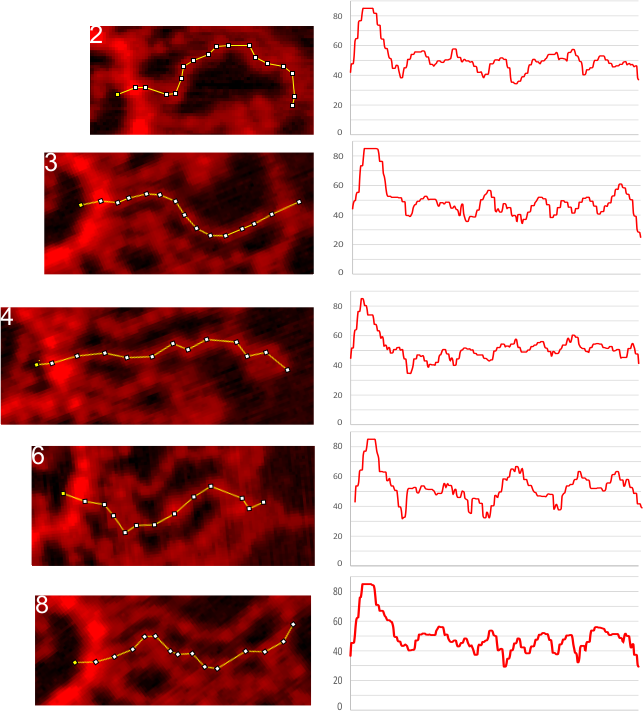
Finding ways to quantify shape, peak heights, widths, and patterns in a molecule which has long arms (100nm+) and lots of flexibility therein has its challenges. PLEASE READ< THIS IS NOT SURFACTANT PROTEIN D and I was NOT prepared by me, but will remain anonymous for the time being.   BUT, here is a section of a molecule which has approximately 30 arms with very definite “beads on a string” appearance.  Not all of the arms could be traced with sufficient (squinting and mental debating) could be deciphered (in fact relatively few remain untangled enough to produce a LUT plot with any kind of predictability. Here is a stack, which facilitates looking at the arm, the actual ImageJ tracing and the plot of luminance (brighness,  — i havn’t figured out which name is the best yet). Cropped and rotated (so that the bright peak is always at the left — and this was the beginning point of the traces, thus the biggest peak is also always at the left) arms are aligned in a column and are all the same magnification and enlargement. The plots at the right are given in the same height as ImageJ scale measured them, but were aligned by nm (100nm) which was a mean length of a trace of several of the straightest and most easily traced arms. No other alignment of the individual peaks or plots was made but picking a “last” peak that is commonly occurring and normalizing that with the beginning of the first peak cold make the interim peaks more easily seen. Hopefully the technique here will prove helpful looking at SP-D fuzzyballs.

There is pretty much a vertical line for a very wide and prominent ‘First peak’ (blue) followed by a regular less prominent peak of lesser height (gray).  Many of the arms showed four peaks before a rise to the second tallest middle peak (yellow).  Two subsequent peaks show up consistently (green and purple) moving to the right. (TOP IMAGE). Five of the easiest arms to plot also have peaks that line up well (BOTTOM IMAGE panel of 5 arms). (the image used was processed as 2DFFT in gwyddion then opened in ImageJ, and traced with a segmented line)

NO clue

I do not have a clue what 2D autocorrelation does in Gwyddion (yet) but it is so odd that it produced this image of an SP-D multimer.  I see the N termini junction, and a concentric ring which is only very faintly visible in the original, and around that ring lateral lines with four blips.  haha.  but no CRD.  Any clues.

SP-D diameters measured as hexamers 135nm seems best

Measuring continuously through a dodecamer from one CRD of a hexamer to another (a node-rich line adjusted for the slighly bent shape of the arms) in terms of length show that over 116 molecules that there is no significant difference in each hexamer’s length (diameter).
137.47+11.4 (n=16) 136.23=10.47 (n=116) The t-value is -0.84948. The p-value is .198249. The result is not significant at p < .05.

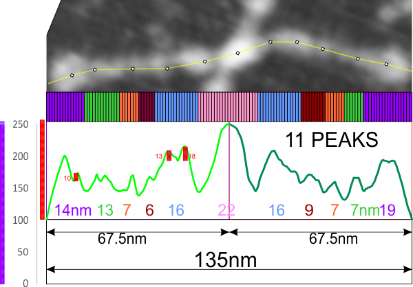
All measures from AFM from Arroyo et al provides me a mean of about 135 nm from tip of CRD to the CRD top on the other side of the hexamer. Nice round number to use to measure distance in peaks.

Count, N: 349
Sum, Σx: 47177.04471
Mean, μ: 135.17777853868 + 11.09
Variance, σ2: 123.14017812959

First new measurements which will be the basis for the remaining 350+ molecules. Y axis is brightness values (0-255, x axis is nm) molecules are adjusted at the N term peak to half of the total 135nm mean from 349 measuremens just from Arroyo et al’s images.

Giving the amino acids colors relevant to their structure

Lots of variation exists on this topic, realistically because of the variations in the properties of amino acids (this is stating the obvious). Not so obvious is the impact of the color schemes given to the amino acids, on the individual researchers who observe them, as they try to figure out if they have meaning. They  respond to subconscious “emotions” and “thoughts” totally unrelated to science, and the colors are conveying “information” about which individuals are unaware.

Case in point, as i looked over the color scheme for amino acids from RCSB, I saw no real order or purpose. Some colors don’t even look nice, and in one case there was a duplicate (since corrected). Also since these colors are no longer what RCSB uses, here comes a new diagram.

A venn diagram described by its maker thusly: “Venn diagram grouping of amino acids based on the biochemical properties: hydrophobicity, size and polarity. Colors for the groups are derived by additive blending of the colors of representative properties.” The blending of colors to create intermediate colors could be better in my “visual” opinion, and I will have to research just how the RGB, or CMYK, or HSL, or whatever they used was calculated (original image uploaded by uploaded by Florian Battke to Research gate). I assume from the venn diagram that the following is more or less what is proposed:
Oranges = hydrophobic

Blue = small
Greens = polar
Blue-green = negative
Turquoise = small polar
Grey = small negative hydrophobic
Pink = small hydrophobic
Brown-orange = hydrophobic aromatic
Orange-pink = hydrophobic aliphatic
This swatch with letter ID is alphabetical, unlike their original which did go by color.

This approach (ref http://www.biomedcentral.com/1471-2105/13/S8/S) calls the method (integrated hierarchical aggregation tables for sequence alignment (with an unfortunate similar acronym with some group about iraq) sorts and displays

Comparing supplemental fig 4 and cover images

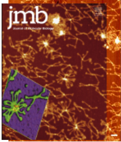
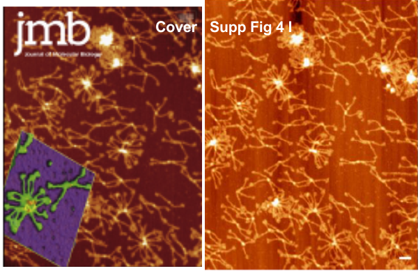
Supplemental figure 4 I is the same figure (almost) as the cover image for Arroyo et al. I see that middle right of figure 4 becomes top middle of the cover figure, thus a 90 degree counter clock wise rotation with a horizontal flip. The figure is cropped slightly to fit the orientation of the cover but since there is no insert the former shows more molecules. The cover image is slightly squished horizontally compared to Figure 4, but I am going to assume that any manipulations of ratio of height to width would have been done in the cover not the original image (probably not a good assumption). Top figure shows the cover in near-perfect alignment with Supp Fig 4, bottom figure shows cover and Figure 4 I side be side. So measures of the cover images can be subjected to morphometry (as duplicates where they are duplicated, and as additional images where they are not previously measured using the Supp Figure 4 dodecamer bar marker. 

Stretchy is good when you are reaching for virus

Just thinking about the odd shapes that SP-D dodecamers (and all other trimers, hexamers, multimers etc) and the flexibility of the three molecules entwined built from collagen like sequences — that provides that long twined stretchy capacity of the SP-D arms, allowing the CRDs to “reach” for the spike proteins “peplomers” heterologous groups of proteins … I did not find the origin of that word but presume it is from peptide and the suffix “mer” or “mere” meaning group.

Two methods for measuring SP-D

1-tailed t-test for seeing if measures of arm length spanning a hexamer, that is from the outer edges of one CRD through the N terminal junctions and out another arm to the other CRD. of a diameter (touching 3 of the four CRD trimers at the ends of at least 3 of the four arms of SP-D (the smallest diameter able to be made).

Previous t-test has not shown a difference, however using all measures to date which includes AFM, rotary shadowed and negative stained images (all available in published documents) there may be a significant difference between methods. Below n=291 arms (which is 145 dodecamers) using the two methods (where n=diameter is
half as many as the separate measures of two hexameric arms.
Difference Scores Calculations

Two hexamers measured with a vector/node line running from CRD to CRD)
N1: 291
df1 = N – 1 = 291 – 1 = 290
M1: 133.8
SS1: 187767.45
s21 = SS1/(N – 1) = 187767.45/(291-1) = 647.47
One measurement of the smallest diameter which touches the outer edge of three of the four CRD.
N2: 146
df2 = N – 1 = 146 – 1 = 145
M2: 127.48
SS2: 82472.16
s22 = SS2/(N – 1) = 82472.16/(146-1) = 568.77
T-value Calculation one-tailed
s2p = ((df1/(df1 + df2)) * s21) + ((df2/(df2 + df2)) * s22) = ((290/435) * 647.47) + ((145/435) * 568.77) = 621.24
s2M1 = s2p/N1 = 621.24/291 = 2.13
s2M2 = s2p/N2 = 621.24/146 = 4.26
t = (M1 – M2)/√(s2M1 + s2M2) = 6.32/√6.39 = 2.5
The 1-tailed t-value is 2.49859. The p-value is .006418. The result is significant at p < .05. The 2-tailed t-value is 2.49859. The p-value is .012837. The result is significant at p < .05 Values from the two measurement approaches when the Arroyo mislabeled nm cover image measurements are removed from each type of measurement Difference Scores Calculations Two hexamers measured with a vector/node line running from CRD to CRD) N1: 261 df1 = N - 1 = 261 - 1 = 260 M1: 128.16 SS1: 104135.99 s21 = SS1/(N - 1) = 104135.99/(261-1) = 400.52 One measurement of the smallest diameter which touches the outer edge of three of the four CRD. N2: 131 df2 = N - 1 = 131 - 1 = 130 M2: 122.42 SS2: 47925.59 s22 = SS2/(N - 1) = 47925.59/(131-1) = 368.66 T-value Calculation s2p = ((df1/(df1 + df2)) * s21) + ((df2/(df2 + df2)) * s22) = ((260/390) * 400.52) + ((130/390) * 368.66) = 389.9 s2M1 = s2p/N1 = 389.9/261 = 1.49 s2M2 = s2p/N2 = 389.9/131 = 2.98 t = (M1 - M2)/√(s2M1 + s2M2) = 5.74/√4.47 = 2.71 The 2-tailed t-value is 2.71485. The p-value is .006925. The result is significant at p < .05