1 (ONE) molecule (AFM image of surfactant protein D) which I call 41_aka_45 ( published by Arroyo et al, 2018)

SUMMARY: 159 different grayscale (LUT) plots of one surfactant protein D dodecamer — as 2 hexamers (arm 1, arm 2)  and as 4 trimers (arm 1a, 1b and arm 2a and 2b) show that personal judgement is still critical for determining the number of brightness peaks along this molecule.

METHODS: 12 image processing programs (listed below) were used to filter, mask, limit range, change contrast, HSL, etc, to enhance the appearance of peaks in this image.
2 programs (listed below) were used for plotting grayscale data (ImageJ (used on almost all images) and Octave/Matlab (occasionally).

5 signal processing programs were used to count the number of peaks in grayscale plots made by a 1px segmented line  using imageJ, with dozens of variations in the  input statements for those signal processing programs.

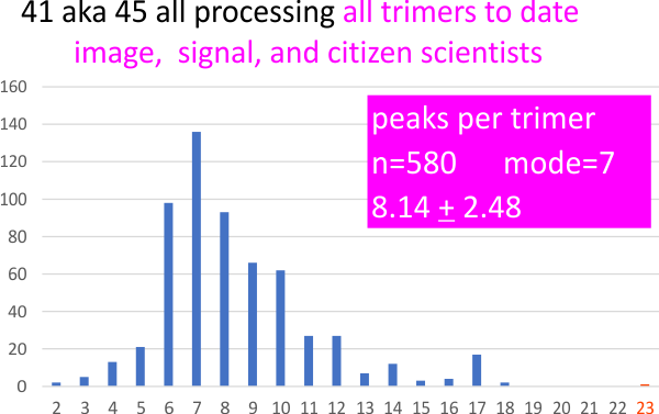
12 peak counts were obtained from volunteers for a single set of plots of this dodecamer (ages 8 – 74  volunteer citizen scientist impressions of the number of peaks).

DATA: All data were saved in an excel file with all image and signal processing parameters to allow assessment of combinations of processing programs and types to produce the most convincing peak counts, widths, and heights.

PURPOSE: To identify a method(s) for assessing the number of peaks, relative peak widths and heights for AFM images of surfactant protein D. (A method that could be applied to countless other AFM application and other molecules).
RESULTS: Nothing produced the results I had hoped for, but there is a clear trend in peak number, width and height. (See next post sometime in the future).
CONCLUSION: Variations in the number of peaks detected in each hexamer produce both an even number or odd number of peaks, the mean and mode are similar,  for hexamers (mean=15 peaks, median=15 peaks, mode is something closer to 13 peaks).  The likely peak number for any given surfactant protein D hexamer is still open, since this is an analysis of methods, not molecules.  The use of this molecule was based on observations of about 100 other images, and represents a reasonable “good choice” to select a methodology.  There are clear options for the most efficient peak detection in image and signal processing, and there are just as clear deficiencies.

A summary of the number of programs, plots and peaks applied to this one molecule is shown below – and it represents the sum total of the data image processing, signal processing, and quick peak counts from citizen scientists, as well as the 100 or so counts of my own, from each image.

Abbreviations:
Image processing programs: psd=Photoshop (proprietary, Photoshop 6 and Photoshop 2021; cpp=corelPhotoPaint (proprietary – raster graphics program, CorelPhotoPaint x5 and 2019); cdr=corelDRAW (proprietary vector graphics program, CorelDRAW x5 and 2019 where the  image adjustment menu was used); gw=Gwyddion, a multiplatform modular free software for visualization and analysis of data from scanning probe microscopy techniques, used here ONLY for image processing; paint=Paint.net (free, open source raster graphics program); gimp=GIMP GNU Image Manipulation Program (free, opensource); inkscape= Inkscape.org (free and open source) vector graphis program; Octave/Matlab (Octave is free and open source) used briefly for image processing (separate from signal processing, limited to 3 plots total, as this was a super cumbersome way to process images). ImageJ, used for both image processing and excel plots (ImageJ is a Java-based image processing program developed at the National Institutes of Health and the Laboratory for Optical and Computational Instrumentation)(free). I added a column of counts of my own, made from each processed image as well (my peak counts).
Signal processing apps: batchprocess  (Aaron Miller’s app for batch processing excel files using  the Lag, Threshold, Influence (open source library); Octave/Matlab (various settings for FindPeaksPlot, AutoFindPeaksPlot, Ipeaks)(check out Thomas O’Haver’s website); scipy, (Daniel Miller’s app for peak finding using Prominence Distance Width Threshold Height (Sci/Python open source library); Two excel peak finding templates – 1) PeakDetectionTemplate.xlsx and 2) PeakValleyDetectionTemplate.xlsx (Thomas O’haver).  Many variations for amplitude threshold, slope threshold, lag, distance, width, smoothing and many others) were used in signal processing.
Citizen science:  Peak counts in a single set of plots of this dodecamer were obtained from a group of friends and family, ages 8 – 78. I did not include my counts in this category as they numbered in the hundreds, not just one set of plots as the former.

Below is just a summary of the number of trimers plotted, in each of the above image and signal processing programs.

Summary of all counts of 2 hexamers, one dodecamer

My counts from the image as processed dozens of times with dozens of filters with the 12 vector and raster imaging programs produced the most consistent results, but very similar to my own counts of the actual excel plots generated by a trace through the center of the hexamers (2 trimers) were found in a manual count of the peaks of plots made in ImageJ.  Both image processing filters and signal processing algorithms have a huge impact on the variation (var) and the min, and max of the number of peaks counted (judgement is required).
It is worth noting that my counts of peaks from the images is the the lowest, meaning to me that processing might be a good backup for confirming what is seen by eye. – In fact, the reason for this study was that I saw a pattern in the peaks (mine more detailed and specific than the pattern reported in the literature), and I wondered if it was provable.

I doubt adding more peak counts to this data is going to change much (LOL). So now, the approach is to separate out the filters, masks, and algorithms which best fit the mean and median.

It is not sufficient just to count the number of peaks in an AFM image of surfactant protein D. That sounds like a rediculous comment but the signal processing programs do just that.  Provide a number of peaks. This just doesn’t help when there are subtle peaks, very prominent peaks, differences in peak width and height, some relative to the height of other peaks and gross variations in the way the trimer (three loosly or tightly bound monomers, depending upon which domain you are looking at and the CRD even with areas which bend over the neck domain in the images which changes the plot lines dramatically.

Similarly, the N termini junction has been  noted as having two different ways for the trimers to assemble into multimers and this too is shown in plots (sometimes two (or three) peaks at the top of the N term grayscale peaks), sometimes just 1 peak.  This likely will sort out in two ways 1) whether the line plotting grayscale goes through a side of the N term junction or through the “center” the latter likely not always “up” in the image.

Sorting the peaks into at least four different categories is necessary when counting up the number of peaks.  In this study, the N termini peak is counted from its valley most distant from the CRD through the entire N term-peak, UNLESS there are TWO distinct peaks (counted by the signal processing algorithms, in which case each half of the whole N term is counted separately.

That way an entire N term length is counted for each trimer, actually with a grayscale plot which always is recorded from N to CRD (regardless of the direction that the protein lies in the image).  The actual line CRD to CRD but the width and peak heights are recorded in the database in order that all calculations can be calculated on trimers, and all calculations begin with N and end with the CRD.

There are programmers who have interests in biology, I am finding, that understand the need for signal processing of repeating and symmetrical pattern-containing signals.  It is an important issue, as there are times when i look at the peaks defined by algorithms (such as Lag, Threshold, Influence) which just dont do what I would like them to do, and as well, there are examples of peak finding (and peak ignoring) which just dont make visual sense to me.  See the plot below (end to end tracing (grayscale plot) of a surfactant protein D hexamer) that has peaks detected using the LTI values using an app made expressly for me by Aaron Miller. It detects lots of the peaks that are obvious, but I am pointing out in the middle and lower images, those peaks which because of the previous values are just ignored, while other peaks which are just tiny bumps in a larger peak, are tagged as a separate peaks.

Top image: blue line is the grayscale plot; boxes are the peaks widths (marked as valleys on either side of the algorithm’s detection of peaks (purple lines); Grayscale axis (y) normalized to 100. This set of peaks in this particular plot (representing one CRD-CRD segmented line drawn through the center of a single dodecamer of surfactant protein D (image is from Arroyo et al). Overall the plot is not very different in terms of peak number than that ascribed to the plot by “citizen scientists” (friends and family) “my counts” (about 500 of them) and various signal processing programs (Octave/matlab peak detection functions); Scipy app (from Daniel Miller), excel peak and valley detection templates (Thomas O’Haver); and an LTI app (from Aaron Miller).

Here are two instances where i don’t like the peaks that are flagged. This sample is from the LTI app (A Lag of 5 will use the last 5 observations to smooth the data. A threshold of 1 will signal if a datapoint is 1 standard deviations away from the moving mean. And an influence of 0.5 gives signals half of the influence that normal datapoints have.) I have put into the link the LTI values for this particular plot.  Two specific instances where i disagree are shown in the plots below, each an excerpt from the complete plots above. Plot excerpt on the left shows one peak NOT detected ( fat red line above the undetected peak), and on the right shows a nonsense (in my opinion) peak (tiny thin red bar above the peak).

RED BARS are over the peak on the left i would LIKE to have detected, and red bar over the peak on the right seems like it should not have been detected. The challenge is to find a model plot and compare the “real plots” to back to the model thus allowing for the extraordinary discrepancies in peak height and width to be tagged, and not removed in moving averages.  The same issues exist in image processing…. but one ends up using judgement, but then, with judgment comes bias.

It is these irregularities that are causing me to go into signal processing for biology with much disappointment.

This has been a long and frustrating journey — and I thank the two kids who have helped me and a retired professor, and other friends and neighbors who have listened to me complain.  The bottom line….

peak finding programs are great at getting rid of noise, but really poor at detecting subtle bilateral peak symmetry

Its almost like I find them unable to get out of their “ruts”, slopes, thresholds, sliding averages for this, and two peaks before this and what about rounded peaks.  Just doesnt work.

Case in point is the enormous number of times I have plotted the same molecule of SP-D and failed to pick up some really tiny peaks beside the N termini junction of a dodecamer, but managed to find 4 peaks on the downslope of the presumed glycosylation peak. I dont doubt for an instant that adding individual molecules to a site in one, two or three strands of a trimer can result in a bumpy elevation, but if the peak finding algorithms find peaks there, then why not the tiny peak burried right beside the very tall, very wide peak for the N termini.  It is like the curse of position.  I could and should at some point determine whether the direction (before or after) the N term peak the tiny peak at the bottom of that valley is ignored or found.  But then it is at the valley between the two largest grayscale peaks in the molecule, right between the glycosylation peak and the N termini peak.  so it is doomed.  And also, not picked up by novice peak finders.  I know this peak is meaningful but how to get it into the peak detection programs is another story.

Symmetry and subtle peaks are just lost in the numbers.

Surfactant protein D is listed in many websites, and even wikipedia, as just the carbohydrate recognition domain and neck domain, little else of the molecule (which includes the N and collagen-like-domain) has been modeled. This blog has many posts dedicated to understanding why the other two domains have not been modeled.

Wonderful images found in Arroyo, et al, offer a great opportunity to look critically at the structure and it is clear that there is much information available from a deeper look at those AFM images.  That was the initial purpose of this blog, however, it became clear that just plotting the grayscale along a line drawn through the images of the dodecamer arms (hexamers) of SP-D some serious processing of the images was required. So I set out to find the “best” that best enhanced the images without changing their data. It also became clear that an unbiased count of the grayscale peaks along the plots of hexamers and trimers) was required. Then numerous signal processing programs were used to find the “best” algorithms for counting peaks.  This, along with image processing ARE still subject to the bias of the investigator.

The parameters for both image and signal processing are driven by the opinion of the investigator, and then I though perhaps some citizen scientists (friends and family) could be asked to count peaks in the grayscale plots to compare to plots from image and signal processing.  The bar graph shows over 500 individual attempts to find the number of peaks in a trimer from a single image of SP-D.  Images below that show the actual image, and an example of one such plot and graph that summary bar graph.

Mean peaks per trimer = 8.14 +/- 2.48 , but the mode is 7, shown below. The mode is 7 likely because when counting the peaks the N term gets counted for each trimer, but is usually seen as one central bright(est) high(est) peak.

White arrow on the image of SP-D shows that the entire N term plus the trimer arm is plotted toward the CRD domain. Known peaks are N, gly, and CRD, the other four peaks are consistent and will be meaningful at some point. The peak at the neck is sometimes seen, often depending on whether one of the CRD of the trimer is lying overtop.

Just from my own observations, there will emerge an additional, very low and narrow peak just at the bottom valley of the N termini peak.  Not shown here, but barely detectable on the line plot (but not marked with a color in the lower bar graph) between N and gly.

One surfactant protein D image, lots of peak number – measurements using various signal processing algorithms.
Just the beginning of the assessment of which peak-finding programs work well with AFM images, are easy to use, and generate more insight than just the opinions of the observers.
There really isnt much new by using these signal processing programs for reasons which I think might be related to the fact that “noise” is a big issue for signal processing, and symmetry and variation are not that well handled. Just a microscopist’s opinion here, not one of a programmer.

Clearly there is still a judgement call to be made on whether to use the “mode or the mean” in deciding what is the best number of peaks.  Differences between the number of peaks on the right and left sides of a dodecamer  (differences in the way the molecule has fallen on the mica, other processing issues) are clearly a stumbling block to a determination of symmetry in peaks, and the slope, threshold and a number of other signal processing options allow for great variability in peak numbers. I am certainly leaning toward the simplest comparison, that of the human eye, and then a plot with modest peak processing to identify peaks and valleys.

To view the actual image (sadly called 41 aka 45) just roam back through the SP-D posts, it appears a jillion times.

There is a section on high and low molecular weight surfactant protein D from an publication by Grith Sorensen in Frontiers in Medicine, 2018 which has the following excerpt. “High-molecular weight SP-D multimers are only partly dependent on disulfide crosslinking of the N-termini, and a proportion of SP-D subunits are non-covalently associated. This allows interconversion between HMW SP-D and LMW SP-D trimers, as demonstrated using size permeation chromatography (36) (Figure 1B). The HMW/LMW ratio depends on the concentration of the protein in solution, with low-protein concentrations favoring the decomposition of multimers into trimers. In addition, the HMW/LMW ratio increases with affinity purification of SP-D, suggesting that ligand-binding facilitates assembly of SP-D trimers into multimers (Reference to an earlier article by the same author).”

There is specific reference to the ratio of high to low molecular weight multimers of surfactant protein D in relation to protein concentration (in the laboratory setting), and to the methionine 11 to threonine 11 allelic variants on the ratio of high to low molecular weight multimers of SP-D in humans.

It seems almost legitimate to view the two different peak plot patterns foud in the N termini peaks, traced from actual images of SP-D dodecamers (traced as two arms, i.e. hexamers – arm 1, and arm 2) found in the N termini of SP-D dodecamers. This valley seen about half the time in the center of grayscale N termini peaks (LUT tables traced in ImageJ) from AFM images (Arroyo et al, 2018) might suggest that even among dodecamers there can be both close tie between N termini (covalent links between two trimers) and loose associations, as well as a single peak, or two peaks respectively). In addition, the trace depends also on “where the segmented line is drawing during the trace, and the brightness saturation of the image.

I am so frustrated with image and signal processing. I dont care what settings (threshold, smoothing, slope -?) are applied. When I see the results of peak finding tags a tiny peak (see red arrow on left)(not so say this isnt an important peak because i think it is — see orange vertical line under that peak) but ignoring a huge, easily seen, not to be overlooked peak massive peak (see red arrow on the right and peak with NO ORANGE line to the peak) I just dont trust any of it.  I understand that slope and amplitude can be adjusted in these programs, but when upcoming and trailing values mess with “reality” (LOL).

COMMENT: this is a plot of a hexamer of surfactant protein D (CRD peaks are on each end, N termini junction is the center peak)

COMMENT: Just think… climate scientists and financial advisors are using similar algorithms to predict doom/prosperity.

11 peaks (brightness/grayscale) traced along a center, 1px line in a surfactant protein D hexamer is the absolute minimum that can be easily described. Furthermore, and routinely, as many as 15 peaks can be found. More are seen with different algorithms, but may not be consistent. Much depends upon how the molecule falls, the over or undersaturation of the contrast (in the original and in the image processing), and the quality of the image (obviously). Also, critical to finding peaks is the care with which the segmented line is drawn (the greater attention to this is what produces two peaks (sometimes 3) in the center of the N termini junction, and in the area just before the N termini junction (i.e. the area between the glycosylation(s) site and the N termini – which i have referred to in several posts as the “tiny peak”).

Thanks to Arroyo et. al (2018). (about 90 images of SP-D) and Thomas 0’Haver and Aaron Miller and Daniel Miller (numerous signal processing programs and algorithms) for their contributions of numerous signal processing programs and algorithms.

11 peaks is just the simplest count from poorer resolution AFM images, using just the most basic image and signal processing tools which are freely available to anyone. But careful analysis and fine tuning images with gaussian, median, mean, sharpening, and range limiting filters, as well as optimizing options such as smoothing, lag, threshold, width, influence, etc  in signal processing shows the peak number to be close to 15+ per hexamer.

One of the surprises of signal processing plots from ImageJ is an apparent disadvantage in peak detection in being a molecule with large differences in peak brightness, coupled with prominent bilateral symmetry.
In the sense of perception of mirror symmetry has significant functions human perception. It has been shown that symmetry is detected within randomly placed elements, and it would be an easy leap to see this visual function as evolutionarily advantageous. Whats more, subjectively speaking, symmetry is apparently pleasing (using self as a sample) as I do this in my own artwork, and see it in architecture and other artwork as well. Not only symmetry but repetition (particularly iterations with rotation) and nature does this supremely well, and it has been studied mathmatically. Instances are too numerous to list and readily available to search online.

An interesting attribute of human sensitivity to mirror symmetry is “tolerance” to error, meaning that variations dont matter a whole lot. This may relate to the extreme abuncance of what biology does with duplicate molecules in arranging them into dimers, trimers, etc on ad nauseum. I am thinking that my interest in surfactant protein D, which has so much “symmetry” (not unlike other patterned, replicated, duplicated, inverted, rotated, molecules found everywhere), and just enough noise may be a visual symmetry puzzle, at best.

What is exciting is that SP-D runs the gamut of everything from monomer to multimer (multimer here being that unique molecule named the “fuzzy ball” by some surfactant protein D researchers, which at any point can have 100 or more monomers). In time, such a multimer will likely show numerous mirror, rotate, iterations which can be seen at quick glance before any image or signal processing.   Just for fun I re-uploaded a graphic mandala that I made a couple years ago, which is a “fake” look at fuzzy ball symmetry (12 trimers, 36 monomers. Alleged glycosylation peaks are a dark blue ring arou the center, CRD are the bumps at the ends of the molecules. Actual SP-D image, masked and colored in CorelDRAW. Pink background, black, white and blue abstract borders are “fills” and not relevant to SP-D structure. Artistically speaking i should go back and edit the background and border for more pleasing texture tile settings and colors. (LOL) and rearrange in the trimers.  Even in this artsie craftsie image the peaks along the arms can be seen. I am not ready yet to relegate the entire interpretation of the shape of SP-D to the best image and signal processing programs. Human input is obviously required still.

Apologetics: I am tired of trying to find a way to calculate peaks and valleys of this protein in a way that might be considered “biasless”.  Great quote I confiscated from a valuable signal processing website gave me inspiration to make a re-do of it.

“image and signal processing do not substitute for judgment, any more than a pencil substitutes for literacy” modified from Robert McNamara.

That said, I have made (with image processing in gwyddion and photoshop) a really nice image of an SP-D dodecamer and so clearly there are about 5 bumps in each of the CRD domains, a funnel shaped bright spot in the neck domains, smaller (and also thinner) peaks along the adjacent collagen like domain, and variable lumps and sizes for the area of the collagen like domain which is believed to be glycosylated.  THe lumps and bumps in this peak area appear to me to be due to the possible partial glycosylation (one, two or three) of each of the trimers.  Then there is the tiny peak which very often shows up right in the valley between the site of glycosylation and the typically very tall N terminal junctions of the four trimers. The latter (shown in this image) has a little depression which is commonly seen in the N peaks dividing that central area into two separate peaks, and even in some cases with a smaller elevation between the two.  All in all, I didn’t need signal processing of the peak plots to see this, and only used the basic filter functions in CorelDRAW and Photoshop to make them stand out.  Lots of effort went into the “image and signal processing” which has taken about two years, and was really not that informative to ME, but was just required to satisfy the predicted onslaught of “bias” comments.

Here is the image described above (41_aka_45, mentioned and shown many times in previous posts on this blog). White arrows and circles point to details mentioned above in obvious places, but all can be found in countless other images of the trimers.