The choice of what algorithms to choose for analyzing 100+ surfactant protein D images (AFM) will amount to selected image and signal processing functions. 6 – 10 plots will be made for each hexamer of a single dodecamer. The concensus plot to which to compare all these plots will come from a concensus of peak number, and peak widths and peak heights from these data. A composite ridge plot created from a single molecule (41_aka_45) (below) indicates that very predictable patterns of peaks and valleys do occur. That said, it is pretty certain that there in an ideal tracing of a trimer there are 7 peaks, and something around 15 in a hexamer (which depends upon whether there are portions of two CRD in the tracing and two peaks found in N (which does happen).
1. maybe two peaks at N
2. two tiny peaks on either side of N
3. The glycosylation peak man NOT be just one peak but a set of rolling peaks – as the number of carbohydrates goes from 1, 2, to 3.
4. a consistently appearing peak peak similar in size to the glycosylation peak located on the lateral sides of the glycosylation peaks, and
two additional,smaller, as yet unnamed peaks, lateral to that peak and before the neck domain.
5. Occasional appearance of a peak related to the neck domain, dependent upon which direction the globular carbohydrate recoginition domains lie during processing.
6. One or two large peaks of similar width and height occur on either end of the hexamer (depending upon the positions the carbohydrate recognition domains fall into as they settle during processing.
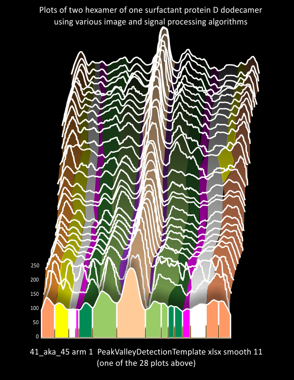
Image processing:
ImageJ for tracing all plots
one image unprocessed
Photoshop 6 for sizing, dpi, contrast and gaussian blur (5px or 10px filters)
Gwyddion for gaussian blur (5px or 10px) and limit range (@100-255)
CorelDRAW x5 for graphics and normalizing plots, dividing plots into trimers,
Signal processing:
one image unprocessed (other images image processed as above)
PeakValleyDetectionTemplate-xlsx-smooth 11
Lag 5 Threshold 1 Influence 0.05 (?Stackoverflow I dont know whom to credit)
Octave, Ipeak M80
Scipy (Prominence 0.2-Distance 30-Width 5-Threshold 0-Height 0)
Data collection:
Excel and Calculator.net
Peaks will be traced as hexamers using a 1 px segmented line, always left to right, and always with an ID of which arm ( hexamers (arm 1 and arm 2), and trimers (arm 1a (always left, and 1b always right, etc). No rotation of the original image will be made (to randomize the traces in terms of possible warping in depending upon the direction of the line as it follows the molecule (this was a serious issue in Gwyddion – but i have not detected it so far in ImageJ), plots exported from ImageJ will be saved, plotted in excel. Screenprints of the molecule, tracing, and plot will be saved as “white paper”.

