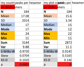
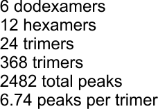
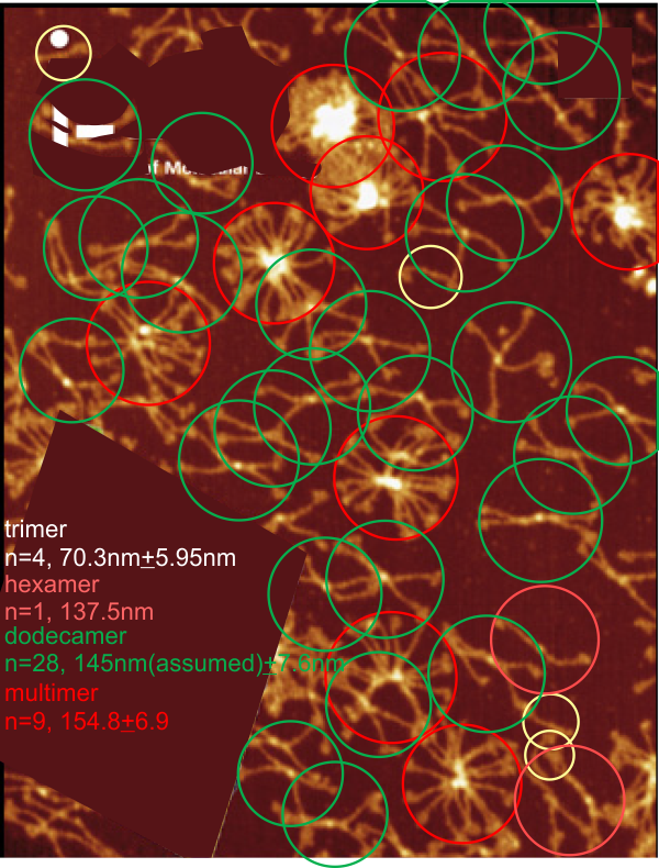
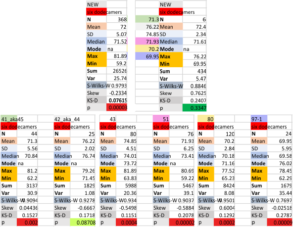
Six dodecamers: SP-D – peaks numbers for trimers, hexamers, with and without signal processing — this data compare the counts of non-processed peaks along a hexamer, with counts of peaks along hexamers which have been 1) image processed or signal processed, or  2) both.

Each procedure i have maintained with its processing settings (for both image and signal processing). Unprocessed images record more peaks that are less likely to actually be meaningful because it picks up individual pixel values which are not always meaningful.

This seems not to be totally alleviated by the use of signal processing scripts. Some identify peaks that are almost too small to measure, worse than picking up pixels.  Since the difference between what is found with image processing (that would be counts from the original plots in imageJ, and my counts from the actual micrograph before any image processing has been made) and also before the image was subjected to any peak finding programs seems to end up a pretty small difference.

This was confirmed by sorting the two sets of data out into “image” and “signal processed” and I had hoped the peak number found in each plot would be greater in the signal processing apps.  Thus i could rationalize it as a way to avoid processing and recording a huge numbers of grayscale plots with signal processing, and rely more on what my own educated guess says about how many bright peaks there are in the four domains of the structure of surfactant protein D.

But there is little consistent difference between the two approaches much to my dismay, the numbers both ways are pretty close.  Maybe both, though are an over-estimate of peak numbers. My personal feeling is that earlier data (15 peaks per hexamer with the odd peak being central N termini junction peak in the hexamer molecule) was a good number, but these last observations are higher.

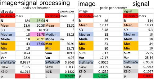
It is also, I have found personally true, that the settings (lag threshold, influence, smoothing etc) are all really individually set….  and while i chose to use the same settings on all micrographs of these SP-D dodecamers (out of focus, light, too much or too little contrast, torn and scratched, lying over debris or other molecules) I could have selected options that made them all fit the way I wanted….. this is disconcerting, as i hoped that signal processing would be the perfect unbiased count…

NOPE. This is a way i had hoped to elimate bias….  but if i change setting on signal processing, i feel it is “bias”,

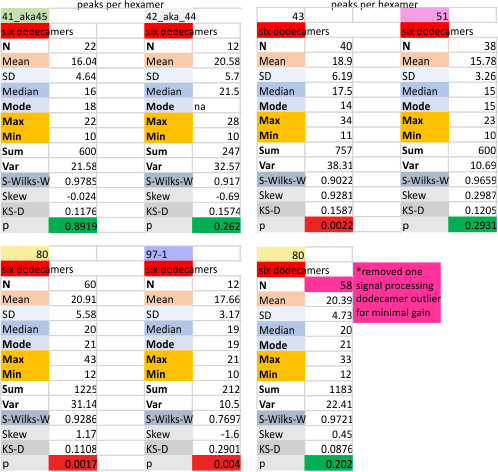
Measures for the 6 individual dodecamers are below( numbers of peaks per each of the two hexamers are listed separately) and from one hexamer ( 80) i removed the hexamer that was suggested to be an extreme outlier using an online statistics calculator for skew. That said, virtually no difference in the mean was seen.

I sense that 15+/- 2  will be the number of consistently found peaks in a hexamer.

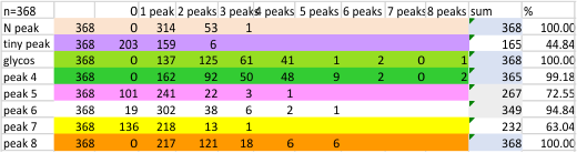
Found yesterday, 5 peaks per trimer (or 9 peaks per hexamer) are noted about 100% of the time.  There are three other peaks present at about 40 60  and 70% of the time that are still in question.

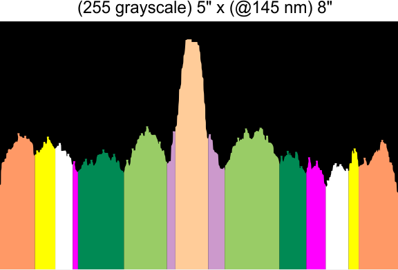
My counts from micrograph and my counts from the original grayscale pleak plots.

Previous signal and image processing programs have shown that the mean number of peaks per trimer is about 8…. this has the N peak counted twice, since the N peak in AFM images only infrequently shows (but sometimes it is very apparent, just not consistently apparent) that there is a decrease in grayscale in the center of the N peak (thus called a junction, as it is the joining somehow of the N term domains of two trimers in the case of the hexamer, and four trimers in the case of the dodecamer).  The number was 15 peaks across a hexamer.

Using that 15 as a guidline, and the signal processing peak finding apps mentioned many times in this blog, i have sorted it into 8 general appearance – type peaks..  That is not individual peaks in particular, but the ups and downs of the valleys and peaks in harmony.  N term junction peak is present in 100% of the grayscale plots (a given), next, the glycosylation peak (peak 3) which is a prominent peak laterally on both sides of the N term peak in a hexamer, is also present 100% of the time.  What I call peak 4 is a rolling but still prominent peak lateral to the glycosylation peaks, and is often wider than the other peaks but also has a higher number of “peak-divisions” than any other set of peaks.  Peak 5 is usually thin, not prominent, and appears just 72% of the time, depending upon how “smoothed” the signal processing app is. Peak 6, is present frequently, measured above 94% of the time, is low and not too broad and it is isolated as a separate peak to justify the division number of 15 peaks that signal processing has defined.  Peak 7 which is pretty clearly the neck region, not present all the time because the CRD domain just flops over and covers it often, and it is quite close and thin, beside the CRD peak. Peak 8 is the CRD peak(s) domain and can presents with up to 5 smaller peaks within what is pretty surely the elevated grayscale values at either end of the hexamer.

Without question, the type of signal processing influences the way peaks are counted, and the settings within those programs.  I will at some point pick out my favorite signal processing programs and use them to recreate the dataset.  CUrrently i like the PeakValleyDetectionTemplate.xlsx (Tom O’Haver), and Octave’s AFPPxy.  These still are not as good as my own peak detection … ha ha…  which i call “educated machine vision”

Six dodecamers: SP-D – an analysis of shape, peaks and size, AFM image, these trimers are not normalized in size (yet) so these values are for each of the four trimers in a dodecamer, and they begin at the (far) furthest side of the N term peak and move laterally to the end of the CRD peak.  This means that each N term is measured as a whole, for each of the trimers. In addition, when we get to peak width, the valley point is on the side of each peak which is proximal to the N term, or maybe a better term is medial to the N term, so the peak valleys are found in mirror images of the trimers, medial in the direction of N term to CRD each direction.  Here is a link to easy measurements (diameter) of dozens of SP-D molecules (Arroyo et al, cover image) and little has changed in the time between when i began working on finding out how molecule size variation of SP-D hexamers in 2019 (btw, the simplicity of this approach is really striking and the image is pretty nice too), and what is seen now in 2023. It is really hard to rationalize the 3 to 4 hours required to make this image, and the 3 or 4 years it is taking to validate those values in an “unbiased” (tongue in cheek) way.  There is no unbiased observation here, just call it science with discretion.  Below, top section is the individual value summary (left) and the n of 6 dodecamers (right) each as an N.  Bottom row has data for each individual dodecamer.

It has been a while since i posted results of my attempt to determine the shape of the SP-D dodecamer (hexamer and trimer) using AFM images (mostly from Arroyo et al). Plotting and finding signal processing programs to do this without bias (of course that was naive, as there is choice in the paramaters of each programs algorithms) took a couple years… but adding two new dodecamers (hexamers, trimers) to the dataset took just a couple months. The data can be compared, the first four, vs the first 6, that is the original four reduced to more or less similar numbers of plots and similar numbers of signal processing programs with two new added.  The latter two will provide the format used for all others.  That is: one image, six different processing methods, the first of which is “without signal and without image processing” the other five using signal processing programs (those selected have been stated before). So these data are the first four fact finding, but trimmed, datasets, and the data from the last two images are provided from what will be the methods for all future plots.

Just trying to figure out how to make these plots tell a story….

Most preliminary numbers are of the hexamer width.  See below: top image was the original set of four. Image below that (six individual dodecamers, listed separately, and with two means for the whole – 1) which includes all plots in a single number (n=1 big dataset), and 2) the data for each of the six molecules individually (n=6). You can compare the initial results with the more refined results… pretty similar.