Purpose: To contribute to predictions about the current structural model of surfactant protein D, in particular, the collagen-like domain.

Aim: To suggest there are recognizable patterns in the number and shape of peaks in grayscale plots of SP-D obtained when traced from CRD to CRD as a hexamer that can inform molecular models. These grayscale plots of recombinant human surfactant protein D (SP-D) were made with ImageJ from published AFM (atomic force microscope) images (Arroyo et al, 2018) of each of the two hexamers which comprise one dodceamer. Images were ploted as unfiltered images, and as images subjected to a variety of image processing filters and/or signal procesing peak finding functions.

Introduction: A single molecule of SP-D has four domains:  N terminal domain,  collagen-like domain,  coiled coil neck domain, and a carbohydrate recognition domain (CRD). Monomers of SP-D are coiled homotrimers which readily form multimers joined at a communal peak at N terminal domains. N terminal junction peak height and width appears to be a function of how many trimers are bound as a multimer. Hexamers and dodecamers are common multimeric forms, though multimers be found with 30+ trimeric arms (Arroyo et al, 2018).

RCSB ( ) (as of this writing) has many molecular models for the CRD and neck domains of SP-D, but none of the full trimer (all four domains) (nor for hexamers, dodecamers or other multimers(   ). Various electron microscopic techniques confirm that the collagen-like domain is reasonably straight or slightly bent, but this information has not yet become part of the molecular model of SP-D.

Arroyo et al (2020) published a grayscale peak count for a trimer at three: 1) N terminal peak, 2) glycosylation peak, and the CRD. Plots of a hexamer would be 5 peaks from CRD to CRD:  CRD-glycosylation peak-N-termini junction peak-glycosylation peak-CRD.  (Diagram modified from Arroyo et al, 2020 check). Certainly other peaks exist, and 3 was a conservative estimate.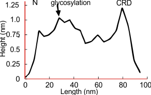
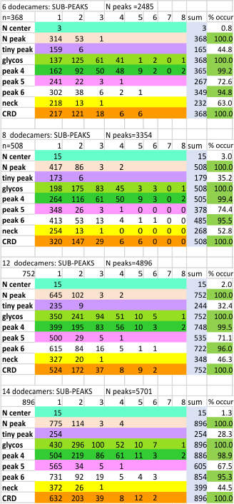
However, a visual count of grayscale peaks from the original 80+ AFM images, and peaks counts obtained from the grayscale plots, with and without image and signal processing functions demonstrated that there are many more than 3 peaks per trimer (5 peaks per hexamer) that are found consistently.  Examination of the raw images, images subjected to image filtering, and peak finding functions, showed the peak count for a hexamers was 15.  Two additional peaks occur less than 50 percent of the time, not included in the 15, were considered “possible peaks”.  The number of peaks per hexamer found without the use of image filters and peak finding functions, was not significantly different than the number of peaks found by just observing the image.

Twelve image processing programs and 4 signal processing programs (each with numerous settings for filtering (e.g. sharpen, median, mode, mean, blur, limit range, noise  reduction, etc., and peak detection (smooth, lag, influence, distance, height, threshold, etc.)) were applied to a representative dodecamer selected to determine which image processing and peak finding apps to apply. Considerations included availiability, ease of use, cost, filtering options, output format,  consistency with with the visual data from the original images. The resulting number of peaks detected (15) using all results was used as a bench mark.

From those initial plots (n=633) a set of  7 imaging programs and their filters,  and 4 peak finding programs and their criteria, were used to assess peaks in 13 additional dodecamers. These data were analyzed individually and together, and demonstrate that 15 peaks are present per hexamer, of which 9 peaks (5 peaks per trimer) were present 95-100% of the time, two peaks per hexamer (1 peak per trimer) were present 71% of the time, while a peak alleged to be at the neck domain was detected 51% of the time. One additional tiny peak was often visible, lying near the valley on the down-slope on either side of the N term junction peak. It was consistent in width, height and location,  and was detected 42% of the time (in this discussion it will be referred to as the “tiny peak”.

The linear aspect of the collagen-like-domain, and the presence of 5 easily detected peaks per trimer, along with their peak heights, widths and valleys should provide useful information for predicting the molecularmodel of the collagen-like-domain of SP-D. In addition, the data show that visual identification of  peak characteristics and number per trimer (and hexamer) of SP-D was not significantly different from data from images subjected to filters.

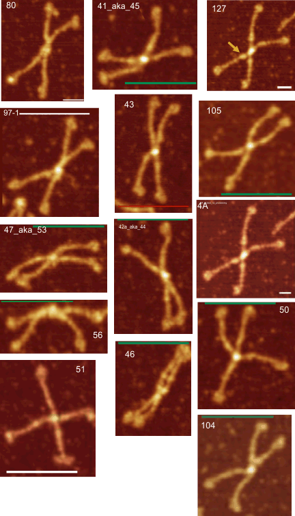
Red arrow (figure below) shows the trajectory of a the trimer (beginning at the bottom, CRD, moving upward to the N terminal domain which is linked to three other trimers at the center of the dodecamer.

Methods:

Peak count per hexamer:  Peak count was obtained initially, using hundreds of plots, both manual peak counting and counts found using an inclusive number of programs for both image filtering (12 image programs) and signal processing programs (7). Results from all initial peak finding functions from all software initially tested and one dodecamer image (my number 41_aka_45) for a total of 633 plots.  These 633 plots were used 1) to define which programs, which filters, which functions produced peak counts most comperable to the peak plots created in ImageJ.  This included the lowest counts from a variety of (unbiased?) citizen-scientists,  counts including poor resolution (highly pixelated) images, images filters and subjected to peak finding functions. This set of plots determined the number of peaks per hexamer to be 15, a number which was also verified stepwise with 4, 6, 8, 12 and with the final dataset (14 dodecamers and selected functions).

15 peaks per hexamer was used as a baseline for assessing the peaks found by plots analyzed in several different signal processing programs and settings. Both counting peaks by hand, and by function certainly carry some bias. It becomes matter of selection of how to apply parameters in many cases even when visually it appears illogical for the inclusion, or exclusion of some peaks by signal processing functions (see post  “to peak or not to peak“.  Images were selected as they appeared within original images, every image that was able to be cropped from a figure was saved, thus limiting any selection bias. Number of grayscale peaks in a single hexamer of SP-D was taken at 15 bright (8.1+/2.4 peaks per trimer where the N termini junction is measured as ONE peak whole peak).

Image processing programs and filters:  Programs used for the initial peak counts (left column), and the programs used for image filtering listed in the right column (which contains free software, as well as two prominent paid programs). Typically the free-ware provided fewer options for subtle filtering than paid programs. ImageJ was used for plotting grayscale values (peaks) exclusively. T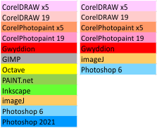he only other program used for plots was Gwyddion and some discrepancies in tracing grayscale when plots were made in vertical directions as opposed to horizontal, however Gwyddion was used for image filtering.  The final choice of software for image filtering is listed on the left.

 

Initial signal and image filtering apps are seen in the top portion of this figure, and final choices for all 14 dodecamers lies below.

Further analysis and fine tuning images with gaussian, median, mean, sharpening, and range limiting filters, as well as optimizing peak finding options such as smoothing, distance, height,  lag, threshold, width, influence, etc  in signal processing shows the peak number to be more than 15 peaks per hexamer.

Line tracings of SP-D to produce grayscale plots:  End to end through the center of the hexamer, segmented line, plotted as grayscale in ImageJ.  Some details here.

Three peaks per SP-D trimer (5 peaks per hexamer,  9 peaks per dodecamer) have been identified. The tallest peak is central in each hexamer/dodecamer comprising the N terminal junction: 1 N-terminal domain for each of the trimers in the dodecamer. Grayscale plots through the center of a hexamer will have N=4 N terminal domains if it is plotted in a dodecamer.   the glycosylation peak(s) (when the SP-D is glycosylated) lie on either side of the N-term peak and the carbohydrate recognition domain (CRD) peak(s), and each of these was recognized by Arroyo et al, (2018). However, their plot (Figure 2, C) 15 peaks can easily be counted, not just the 5 peaks per hexamer that were listed (a very conservative count) in their legend. After extensive analysis, 15 peaks is a reasonable number and, in addition corroborates peaks on their initial plot.

and peak visually from unfiltered images before plots were made (group 1 ) a visual count of bright peaks (arm a in figure 1). Grayscale plots were made (using ImageJ) to determine peak number, height, width and valley of those same unfiltered images by drawing a segmented line lengthwise through individual hexamers (2 per dodecamer) beginning at one CRD through the center width of the N termini junction peak and continuing to the second CRD) (figure 1 yellow plot line, arm b)( a count of peaks from the ImageJ plot.( group 2) .  Each of the plots were were then subjected to signal processing functions (group 3) to compare (confirm?) visual assessments (eliminate bias?). LEGEND: Surfactant protein D dodecamer. Two hexamers, with each hexamer of the dodecamer labeled as arm a or arm b. CRD at bottom, center, bright spot (labeled START), moving in the direction of the white arrow to the bright spot at the top of the image (the CRD at the other end of the hexamer). .  Red arrow shows the extent of a trimer plot, from CRD (at bottom labeled START, through the entirety of the brightest peak (N termini junction).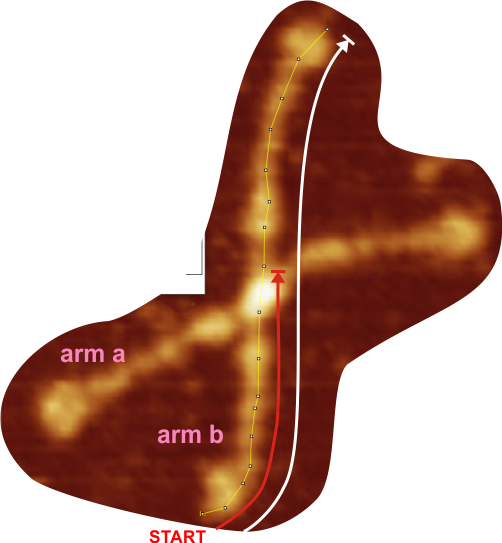 

Total number of plots examined for 14 SP-D (figure 2) dodecamers came to over 1500 trimers (that is 385 dodecamers).  14 dodecamers were thus, plotted about 100 times each. (see number for each different dodecamer below.  The largest numbers were those several dodecamers that were used to establish the mean number of peaks per hexamer. Clearly dodecamer labelled 41_aka_45 was used to determine which image filtering programs, and which settings for signal processing filters would be used for the other dodecamers. The list also shows the image of each of the 14 dodecamers (labeled in white on AFM images.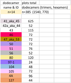  

Molecules numbered 127 and 4A are the same but derived from different figures in the same publication. Bar markers in the images varied in the figures from 20,30 to 200nm. Each image was manipulated “along with” its bar marker to insure that dimensions were consistent.

 

A list of image filters and signal processing functions: (41-aka-45) 292 different image filters plus signal processing functions (trimers so n=73 dodecs)  332 plots, all different image filters in x different image processing programs n=83 dodec)

Image processing programs and filters

 

 

 

 

Training: the dictionary defines training as  “the action of teaching a person or animal a particular skill or type of behavior”. That definition now includes computers and each comes both with great potential, and great limitations.

Learning: the dictionary defines learning as “modification of a behavioral tendency by experience”, and in the case of artificial intelligence, to learn without explicit programming.

Bias: the definition relevant to research is “systematic error introduced into sampling or testing by selecting or encouraging one outcome or answer over others” or “a disproportionate weight in favor of or against an idea or thing”. A rather negative view of bias in research (Zvereva and Kozlov, Sci Rep 11, 226 (2021)DOIhttps://doi.org/10.1038/s41598-020-80677-4), but suggest two important approaches to limit bias – 1) understand the measures available to avoid bias and 2) report measures used to avoid bias. They also state “Cognitive biases are unconscious, which means that simply being aware of the existence and importance of biases is not sufficient to avoid them”.

Machine learning bias: “Machine learning bias, also known as algorithm bias or AI bias, is a phenomenon that occurs when an algorithm produces results that are systemically prejudiced due to erroneous assumptions in the machine learning (supervised and reinforced machine learning) process.”

(it seems like unsupervised, supervised and reinforced machine learning should be great backup for limiting bias in interpretation? – aka mistakes, selection bias?  in a relatively simple assessment of peaks in a given plot.

Bias present:

1) non-response bias (missing value): “As a rule of thumb, the lower the response rate, the greater the likelihood of nonresponse bias. Nonresponse bias becomes an issue when the response rate falls below 70%.” (says who)
2) automation bias: “Automation bias is an over-reliance on automated aids and decision support systems”. (method bias)?
3) in-group bias: ” the tendency for us to give preferential emphasis to one group, while ignoring outgroups”.
4) implicit (unconscious) bias: automatic and unintentional, yet impacting outcome (judgement)”.
5) reporting bias: “the decision about what to report depends on the direction or magnitude of the findings”. (thats what peer review is for)
6) false impression bias: “also known as the frequency illusion or recency illusion”
7) sampling bias: “a type of selection bias” –( e.g. test molecules being systematically more likely to be selected in a sample than others).
8) selection bias: “selecting an item (or various items), not using randomization of those items. therefore the data is not representative of the given population”.
9: confirmation bias: “the tendency to search for, interpret, favor, and recall information in a way that confirms or supports one’s prior views”
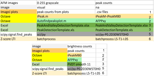
10) measurement (data collection) bias (errors): ” refers to the tendency of algorithms to reflect human biases (supervised and reinforced machine learning), (personal communication : “you chooses the settings” which is true for python-scipy peak finder (prominence 0.2, distance 30, width 5, threshold 0 height 0); for PHP Zscore (Lag 5, Threshold 1, Influence 0.05), for Octave’s AutoFindPeaksPlot.m (xy), ipeaks.m (M80), and also in PeakValleyDetection.xlsx (smooth 11)).

Bias relevant to outcome,

Selection Bias (yes, just dodecamers, from one researcher)
Spectrum Bias
Cognitive Bias
Data-Snooping Bias
Omitted-Variable Bias (missing data)
Exclusion Bias (out of focus molecules)
Analytical Bias
Reporting Bias (this would appear to be an ethical issue)

The definition of all of the above words has changed: in society, in science, in philosophy.
In the context of this post, the To create an “unbiased” count of the number of peaks

“people should assume right now that the models only perform to about 95% of human accuracy.” (https://mitsloan.mit.edu/ideas-made-to-matter/machine-learning-explained).

Results and Discussion:
Peaks, subpeaks. Figure below shows the analysis at four different tiers in analysing the number of peaks and subpeaks in dodecamers: as an N= 6, 8, 12 and 14 individual molecules, each processed in many ways, and each included  in subsequent analyses.
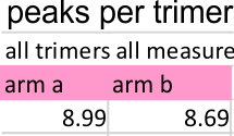
Peak number per trimer is shown in graphic below of an analysis of 14 trimers shows there is no statistically significant difference (none was expected either since SP-D should appear as a bilaterally symmetrical molecule ) between the number of peaks in either of the hexamer’s arms (a and b, i.e. left and right sides of a hexamer, respectively) and therefore, of any trimer in a dodecamer.

References and links:

1. Arroyo et al, 2018, https://doi.org/10.1016/j.jmb.2018.03.027

https://imagej.nih.gov/ij/
https://terpconnect.umd.edu/~toh/spectrum/PeakFindingandMeasurement.htm#ipeak
https://terpconnect.umd.edu/~toh/spectrum/PeakFindingandMeasurement.htm#findpeaksx
https://terpconnect.umd.edu/~toh/spectrum/PeakFindingandMeasurement.htm#Spreadsheet (s)
https://docs.scipy.org/doc/scipy/reference/generated/scipy.signal.find_peaks.html
https://stackoverflow.com/questions/22583391/peak-signal-detection-in-realtime-timeseries-data/22640362#22640362 (version: 2020-11-08)