Category Archives: Methods to assess TEM and AFM images

8 dodecamersL SP-D: Subpeaks per peaks detected using AFM images of surfactant protein D.

8 dodecamersL SP-D: Subpeaks per peaks detected using AFM images of surfactant protein D. (APOLOGETICS) Always and at the outset I thank Arroyo et al for the 2020, 2018 publication of the SP-D AFM images (the best I have encountered of SP-D), and secondly I thank Dan Miller for the scipy app for peak finding, Aaron Miller for the LTI app for peak finding and batch processing, and Thomas O’Haver for his help with Octave, and excel templates, and also for ImageJ and Gwyddion (and I guess i should be very grateful for the original developers of CorelDRAW (which was Kodak)(not the new owners as they get a thumbs down from me), and also the original producers of Photoshop (yep, version 6 on CDs performed just as well for image analysis as rented versions of 2021 (so it is also thumbs down to them)).

The following is the result of 508 image and signal processing plots of 8 images of surfactant protein D. These data are reported as individual plots of hexamers (thus four trimer plots (as separate entities, with plots beginning at the full width of the N term plot and progressing to the CRD.  I have made the assumption (which I will discuss) that signal processing algorithms are smart enough to see symmetry… bilateral symmetry, which apparently is giving that AI too much credit.

Notwithstanding that problem, the total number of peaks per trimer (8) established some time ago is the number which is used to box the number of subpeaks into 8. Below are the data for 6 dodecamers (n = number of plots analyzed, not the number of dodecamers analyzed) and 8 dodecamers. Consistency is apparent. Not all peaks show up 100% of the time. Peaks such as the N and glycosylation and peak 5 and CRD peaks are often lumpy (meaning they have subpeaks.

There is a peak called “?” which only rarely occurs in dodecamers (but in my opinion is frequent in multimers (called fuzzy balls) and is indicative of a side to side N term association among molecules. It is reasonable for that peak NOT to show up below.

The N peak is present 100% of the time, as is the CRD peak and the glycosylation peak (though the height of the glycos peak varies (and at this point unglycosylated AFM images of SP-D have not been analyzed, so that will be dependent on the SP-D molecule, which species, and mutations and other factors, but here it is rhSP-D). Peak 4 is very consistent, present 99+ percent of the time, not previously reported, lying in the collagen-like domain. The next two peaks have characteristics that are obvious visually, peak 5 is not wide, and is not tall but consistently shows up right after peak 5. Peak 6 is broad, and appears regularly (94+ percent of the time, and is also low.  Peak 7 is what I believe is the neck of the SP-D trimer, and it is very often covered by the bright peak of the CRD (and this depends on whether the rounded ball shaped CRD peaks are positioned directly over the neck or to one side.  (Just my opinion here).  The glycosylation peak and peak typically have more than one subpeak.
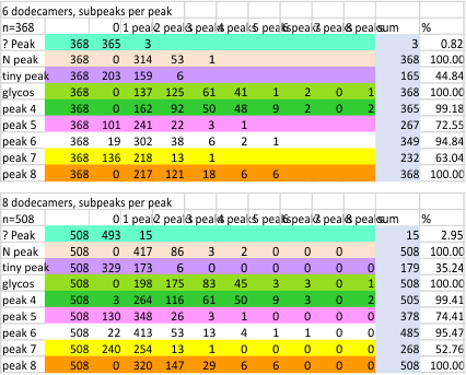
8 dodecamers of SP-D

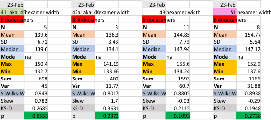
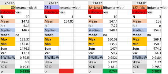
Two sets of measurements have been added to the dataset for hexamer (that would be the CRD to CRD measurement of two trimers with N terms meeting in the center of the dodecamer) (Numbers of the molecules are my assignments  (out of about 90 different images) and number 127, and figure 4A,  are both images of the same molecule, but found in separate figures from Arroyo et al). Different image processing apps have been applied to strengthen the signal from the peaks from all images, and each image then was subjected to signal processing peak findings (5 different apps and settings which are now used for on all plots of images).

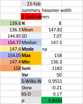
The data for hexamer width have really changed from previous analyses, i dont think more will be useful in determining the hexamer width.  I will still do this (just to find outliers and potential mistakes) in the upcoming images that I analyze.

Early data is on this blog….  you can check if you like.

Feb 23 data with 8 molecules processed in almost 900 different plots is summarized below.  The diameter and the length of the arms is calculated separately (in nm, relying on the nm bar markers in each image used).  THe total number of times the hexamers are measured is less than the total number of times the trimer widths are plotted since the same image is used for the signal processing (thus repeating it, while it makes very little difference in the statistics) has not been done here.

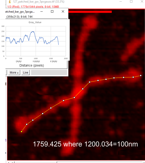
Tiff image from Gwyddion as R, indexed to tiff RGB in imageJ, grayscale plots — same x but different Y

Dilemma:  How to use the grayscale plots of SP-D hexamers obtained in ImageJ from images exported from Gwyddion (as red only) in the same datasets as imageJ plots of SP-D hexamers obtained from tiff files exported as RGB.  ???  I have left out of my peak height and valley analysis all those plots from Gwyddion because i did not know how to use them. They have very low grayscale peak points and can’t be used along with those which have a highest peak grayscale value (RGB) of around 250.  The peaks at about 90 (0-255) and peaks at about 250 for both types of plots just dont work together and I hate to ignore the plots from Gwyddion (as they have a good  “limit range and gaussian blur” filters).

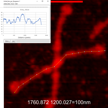
To see if  I could safely adjust the plots required figuring out, in ImageJ, how to save a segmented line drawn in an image saved in R only, and recall it, and use it on an identical image saved in RGB.  So I did this, and while the two plots are not totall “identical” as i moved one node at the right end, they are almost identical. Each grayscale line plotted in imageJ for the R and RGB image was saved to excel. (i wish i could figure out how to create a standard plot template in excel, because even if i choose 0 to 255  scale in ImageJ, excel does what it wants with the y axis and i have to rescale it.)

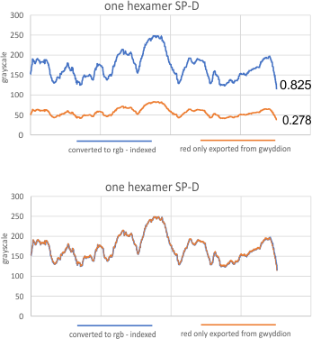
Below are images of the identical SP-D image (named 127 aka supplement 4A) exported from Gwyddion (gw) as a red tiff, and plotted, and changed to indexd RGB in imageJ, and plotted again using the same segmented plot line restored.  Both plots were saved, and opened in excel and a chart was created. Those two plots were saved as metafiles and pasted into corel draw, ungrouped and the line from the R only plot was scaled (without rescaling the x axis) to the same height as the plot from the RGB image and then moved to bottom right of the RGB plot.

As you can there is no difference between the R and RGB plots.  So this means to me, that i can take my gw plots and scale them on the y axis and use them in my dataset with the RGB plots.  Any issues that i am missing that say “dont do this”?

Top two images are the images with segmented plot lines created (and saved) in imageJ. Bottom image is the two plots, and the lower plot scaled to the y axis (only) and pasted into the RGB plot. — so the difference in grayscale peaks can be scaled using a formula.


Indeed it would be almost laughable if it just requires a 300pc increase, i would need to find the grayscale value for the highest peak of each image i think inorder to align the R plot to a value.

Thanks to my kids…. dan and aaron. Dan was right in seeing that the grayscale R image max grayscale value was 85.  i will use a factor of 3 when analyzing the other gw plots to find a grayscale comperable to the RGB plots.


SP-D new way to show ridge plot and grayscale peaks

Still working on the peak height, width, valley measurements on surfactant protein D dodecamer grayscale values using AFM images.  Just thought this was an interesting way to show both the signal processing divisions for peaks, as well as the more subjective estimation (also from peak counts of image and signal processing peak numbers) division into sections. N peak center, either side, glycosylation peak(s), next is a long lumpy section (dark green), a reasonably consistent tiny low peak (pink), and a broader peak before the presumed neck coiled section (white), the likely neck domain (yellow) and the CRD (orange).  These measurements are taken from the N term outwards in two directions to the respective CRD of hexamers.  Two hexamers are measured separately, though mirrored and identical (theoretically) in all for trimeric arms.

This particular ridge plot is from molecule 80 (my designation number, as collected mostly from images found in Arroyo et al), and light gray lines along the plot lengths for each of the two hexamers are the divisions found by octave’s ipeak.m program using M80 as the amplitude and smoothing settings (unbiased).  These come close in this randomly selected image to fitting the 15 peak per hexamer consensus found previously. Color divisions are mine (educated bias), made to approximate the 15 peak per hexamer findings as well as my observations on the AFM images.

An obvious deviation is the unusually tall (bright) peak on the left side of the top hexamer at the domain of the CRD, and just as unusual is the low (less bright peak) on the left side of the bottom hexamer.  In other respects this molecjule (number 80) is very close to the means found for the first four dodecamers posted on this site.

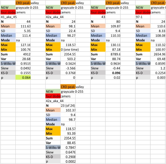
Four dodecamers: CRD peak-valley grayscale values

same MO. See from bottom image that just one of the dodecamers (number 42a_aka_44)  had any missing values, and then just 1. So the separate sum (172 with and without that one missing value) is listed in the top image, along with the summary of just the means of the four dodecamers calculated separately) and the single dodecamer with one missing value is the very bottom set of valley parameters.

Four dodecamers: values for the valleys of peak 5

SP-D peak widths, heights and valley values for four dodecamers. These are the data for peak 5. (count begins with peak 1 as the N term peak and moves toward the CRD, each for trimers.

When there are peaks which are “not detected” a value of 0 was used, and data were plotted both ways, i.e. with the non-detected and eliminating the non-detected). The pattern was applied to all peaks as one dataset, and to individual dodecamers (N=4) – see bottom image.

Four dodecamers: peak 4 “valley” grayscale values

The peak just lateral (remember going to the right and the left of the N term peak with peak 1 being counted as the center N term peak), peak 4 is a very consistent finding with image and signal processing. You can see top image shows that only once in 172 plots of trimers was there no detection of peak 4. Means and other data are shown both ways. The image just below that is the mean grayscale valley value for peak 4, calculated as an N of the number of dodecamers examined, and the N of plots is not the same in the dodecamers, but each dodecamer is given the same weight in those means and SD.  With and without the single missing value in one dodecamer, means are very close, that is grayscale value of 112. The third image down shows the mean grayscale value for the peak 4 valley for each of the four dodecamers individually (these were used for the means shown in the second image from the top). Lastly the single dodecamer where a single peak 4 was missing is shown at very bottom).

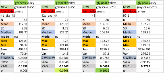
Four dodecamers: glycosylation peak valley

Grayscale values(0-255) the y axis. Glycosylation peak was detected by image and signal processing algorithms 100% of the time, so there is a single value recorded for the valley (immediately lateral to the “tiny” peak – keeping in mind that this molecule has bilateral symmetry beginning in the center at the N termini junction peak. so many images of this molecule have been posted on this blog that they shape of the AFM images is easy to see.