This is a screen print (originally from Arroyo et al, a dodecamer i call #51) boosted to 300ppi in photoshop, and a 3px gaussian blur added, minus-8 points in contrast, opened in gwyddion and a limit range filter applied… 100-220.  It might be my imagination, but i can see very clearly the peaks along the collagen-like domain and even details in the CRD which look so like they could be the three arms of the trimer spread apart at those ends of the molecule.  The glycosylation sites (near the junction of the N termini in this dodecamer) have texture and shape as well, possibly providing information on how many of the arms of each trimer are actually glycosylated.

There is a twisted look (as one would totally expect along the collagen like domain that is distinctly present in two of the four trimers.  Fanning out of the CRD in the lower right portion of the image is pretty amazing. In addition, the one tiny little peak that I am hoping to verify on the downslopes of the N termini combined peak is pretty nicely seen on the left middle of the center of the dodecamer.  There is a little stretching on the trimer on the left center….  moving the glycosylation portion to the CRD just a little far from the N termini group… it is possible that is why the minor peak on the downslope of that side is visible.

Also interesting in this image is the relative decrease in peaks in the collagen like domain in the area past the glycosylation peak but before the neck and CRD (where the twisty look is also evident).

Would it be so unusual to have shape follow the number of glycosylated arms in the trimer of SP-D.  Just look at these two peak shapes.  They are certainly not the same.  Artifact from position and random events in processing can affect this i understand, but it seems to me that for sure peak width will increase with number glycosylation sites (1, 2, or 3) if in fact SP-D is glycosylated in that manner???  I have not read anything to suggest it, or to refute it.

Figure below: same image right and left, plots traced in ImageJ, the width of the glycosylation peak on the right hand trimer of the horizontally running hexamer is clearly of greater width.  RElative peak height may be indicitive of level of glycosylation as well, as it has been reported by Arroyo et al,  that the peak that is assumed to represent glycosylation is greatly diminished in de-glycosylated trimers .  Open to suggestion here.

IN this set of data there are (‘ or is’ – to use the noun as a ‘group of data’ (the latter is probably correct – “Merriam-Webster entry for “data,” notes that both singular and plural constructions are “standard” in English. and as someone posts… “anyone who ‘corrects’ you for noncount use of ‘data’ is being pedantic (and probably rude)” LOL, peak numbers along two hexamers of SP-D.

One image of a single SP-D dodecamer (which i call #51) (from a publication by Arroyo et al) was image-processed with 16 filter variations coming from a half a dozen programs,  then analyzed for “peak count” (or “LUT” peak count (aka  “grayscale 0-255 brightness”) by 2 visual and 6 different signal processing algorithms. The purpose is to determine how reliably the number of bright peaks along molecles can be counted in traditional AFM images.

Image processing does change the counts somewhat, but in all plots there are similarities in relative numbers and sizes of peaks regardless of the graphics programs and signal processing algorithms.

The two arms of this dodecamer (51) are clearly different in terms of arm length (artifact likely from stretching and twisting as fell onto the mica). The arms are significantly different in the number of peaks per hexamer.  One could think that stretching one side of the dodecamer could be useful artifact, since squishing of arms would obstruct definition between and among peaks.

Peak values were obtained as follows using the original images processed with 16 different  filters. Filter names are given below: Clearly the filters that increase contrast or mask outliers show different results.

1. Visual count (by eye – after each processing filter
2. Quick count of the peaks in the LUT plots obtained in ImageJ plots (no background subtraction)
3. Batch Process – (an app for excel files that uses dispersion peak detection to detect peaks in the LUT plots obtained in ImageJ) – (lag=1, threshold=0.5, influence=0.025)
4. Batch Process – (lag=1, threshold=0.1, influence=0.01)
5. ImageJ – Find Maxima>0.5>strict>single point
6. ImageJ – Find Maxima>1>strict>single point
7. ImageJ – Find Maxima>2>strict>single point
8. ImageJ – Find Maxima>3>strict>single point

Methods 1, 2, 5, 6, 7, and 8 use the image directly, while Batch Process uses the excel files from LUT plots.

Top figure = image processing filters

The color of the dots indicates which program was used to count peaks, and the number on the x axis corresponds to the way the image was processed before peaks were counted.

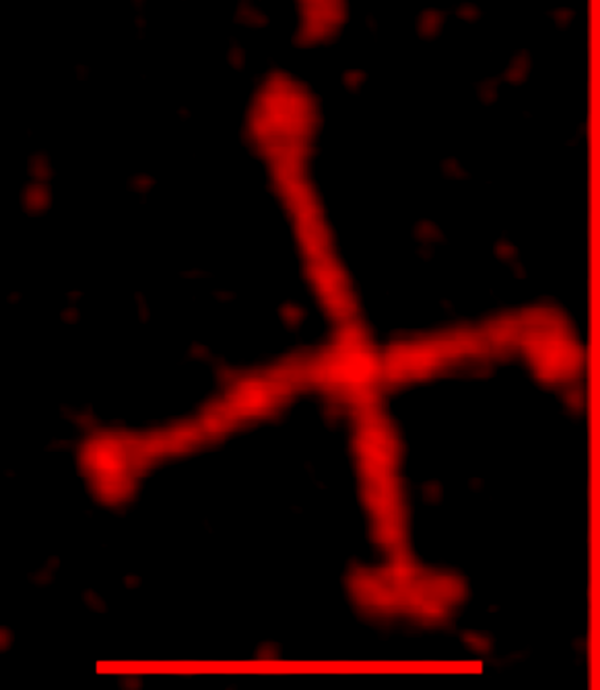
SP-D dodecamer (from Arroyo et al) above.  Arm 1 = middle left to middle right, arm 2 = top middle to bottom middle-right.

Interestingly, my eyes see more peaks than are found with image processing.  And second to that is the number of peaks that appear in the LUT plots (ImageJ) in a quick count (without subtracting background).  Summary counts or all processing (hexamer 1 and hexamer 2)  are probably pretty close to reality.

I need to find out what ImageJ uses for finding maxima … and find a good definition for Lag, Threshold and Influence.

Just an aside….. It took me an insane amount of effort to learn the programs, and to obtain and organize these data (and i need to add Octave to the list of programs)… LOL, but i think they are robust enough that using the same (or similar) scripts on numerous arms of SP-D and DMBT1 will be valuable in sorting out the LUT number of peaks per trimer.

Were I going to choose three methods to analyze additional molecules I likely would choose:  5, 6, 8, 11, and/or 16 for image processing,  then Batch Processing LTI 1, 0.5, 0.25 and ImageJ (Find Maxima 1 strict) for peak counting.

Using CorelDRAW19 various processing algorithms have been applied to one AFM image of surfactant protein D. This image was derived from Arroyo et al, and is among dozens of images from various authors that I am using to test the validity and efficacy of such image processing. The list of programs used for this particular image (then vary from processing programs, e.g. photoshop, gimp, gwiddion, imageJ etc. because of the menu options in each program) and from free and proprietary image processing libraries that may or not be available to software developers. While it has taken months, the comparison is something that I needed to do since I have both old and new versions of the industry standards (CorelPhotoPaint, and Draw, and Photoshop) and it was important to see whether there were changes in image processing algorithms that caused significant differences in gray scale (y axis) for surfactant protein D images.

the list for this composite (plot) overlay is: gaussian blur (5px); gaussian blur (5px) and high pass 40%-10 px radius; gaussian blur (5px) unsharpmask (300%-  20 px radius- threshold 50; lowpass 100% 10 px radius; maximum 50% 10 px radius; median 5 px radius; minimum 50% 10 px radius; smartblur 50. Each of the resulting image were measured using ImageJ. Plots were conformed to the mean arm length of all processing and measuring for this single image.  A single background measure (each background was taken at the same time as the measurements, and in the same location) is shown around 50 on the gray scale.

Each plot is a different color and each arm (meaning CRD to CRD in a hexamer) were plotted separately and are shown separately  thus, 16 individual plots and 16 colors. Approximate width at the valley of the plots is given in nm.