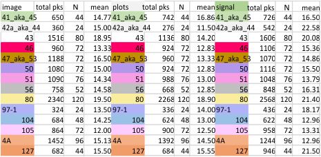
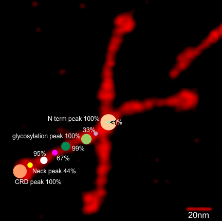
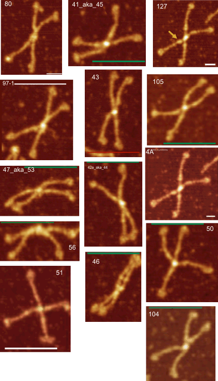
14 dodecamers of SP-D: Width in nm of all peaks. Image below is a thumbnail of each of the SP-D dodecamers used in this analysis (number designation are my own, but bar markers for calculating magnification come from the original publication(s)(Arroyo et al).  All AFM images used (fir the data below) are rhSP-D. Dodecamers labeled 127 and 4A are the same molecule from obtained from different figures within the publication (deliberately used for comparison measures) all others SP-D molecules are unique.

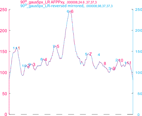
The total number of peaks (traced using the segmented line option in ImageJ) has been shown many times to be just over 15 peaks per hexamer of SP-D. And the segregation of the various peaks plotted in ImageJ into a 15 peak-category has been largely influenced by my own 1) general assessment of the general shape of the plots, peaks and sub-peaks, and 2) the obvious mirror symmetry of the hexamers (and trimers) of SP-D.
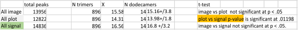
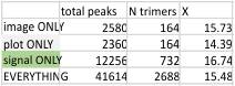
Total number of trimers measured is 896 (14 dodecamers, with many processing apps and image filters). Trimer measurements include the entire N term domain peak in each, and hexamer measurements include each peak appearing from CRD to CRD.  Data could be adjusted somewhat if the arm of each trimer in a hexamer were normalized to a known distance in nm from a center point in the N term domain peak. This has not been done yet in these data.

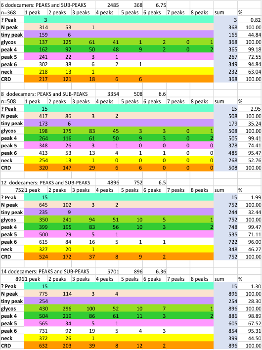
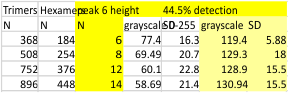
Mean peak width is based on plots made in ImageJ, of images subjected to various image processing and peak counting apps. Summary of progressive analyses (6, 8, 12 and now 14) shows that little has changed since the first measurements. At this point most of the data is derived from signal processing functions (5 signal processing functions vs my 1 set of counts from the images), and while these are purported by some to be unbiased, it must be recognized that I choose the function settings that I think best fit the image.  Largely, the signal processing is “similary biased” to image processing filters and personal observations.  Graphics below show the  mean peak width in nm +/SD for each progressive analysis. Peak  % detection rates for all peaks is found here) or mentioned below.

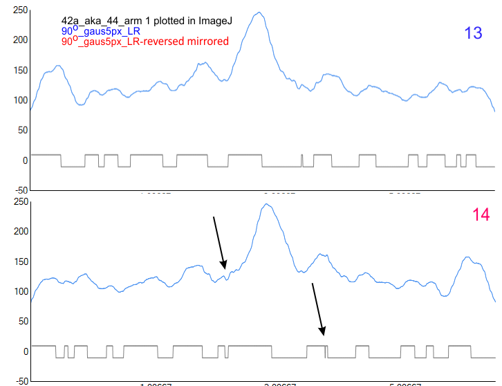
I have added this “iffy” peak data (mint green below) because I really do think it exists sometimes. It exists as a detectable depression or division within the center of the N term junction of just 3 of the 14 the dodecamers (a mere 15 times out of 896 plots) by the signal processing functions, but I see it more often than that. I find a similar low detection rate by signal processing functions for the tiny peak on the downslope of the N term junction peak (which i call “tiny” peak).  Sorting the data by my assessment and all other assessments should point this out (future project).

While I also have observed what looks to be side to side attachment of N term domains in hexamers, most frequently the N term peaks looks to be an end to end attachment — where sometimes there is a decrease in grayscale values (peak height)(thus forming two peaks). How often this is detected by the ImageJ plots is very much dependent upon how I trace the line within the center (lengthwise) of the hexamer. In multimers of SP-D, the center N term peak depression is very often pronounced. Data below show it is infrequent, and narrow in width, as a very shallow depression at the tope of the N term peak.

How much the presence of this peak in the center of the N term peak influences the total peak number is probably minimal.

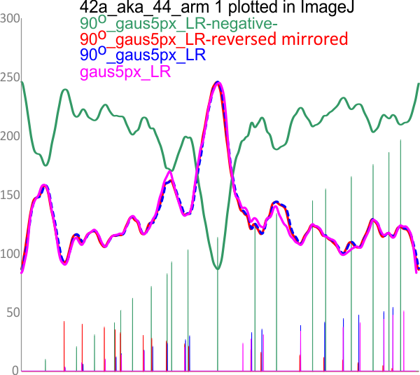
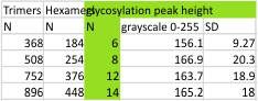
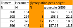
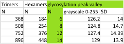
The height and valleys of peaks in the plots of SP-D dodecamers is a measure of grayscale (0-255). THese values are determined by ImageJ for each of the plot lines (two lines plotted per dodecamer, from one CRD of one hexamer to the CRD at the other end) of the images, unprocessed, or processed by a range of filters in a range of programs (link to the exhaustive list of filters and functions tried). Five signal processing functions and two filters  were used most commonly and were selected for the output which most resembled what I saw in the images).

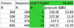
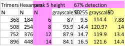
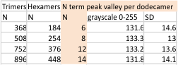
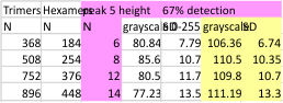
Peak height of the N term junction peak (central in the hexamer) data from four different summar datasets. The bottom row is an update and inclusive of the top three rows (as is true for data above).  The data with the yellow columns are the means and SD ONLY for detected peaks, white columns are for all data for that group. Actually it is nice that peak from 14 molecules plotted with many variations show similar outcomes.
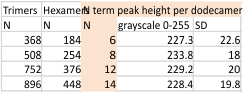
The mid N peak width is so tiny as to not maybe be worth making a graph for. I will decide.

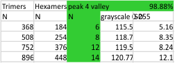
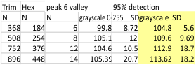
Peak valleys for each of the 15 peaks per hexamer.

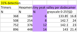
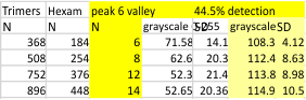
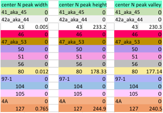
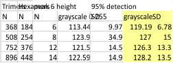
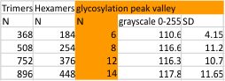
The image below is just of the very rare center blip in the N term peak which i have often mentioned as being prominent in the multimers greater than the dodecamer. This peak is detected in only 3 of the 14 images, and peak width (in nm) and peak height and valley (grayscale 0-255) are shown here.

Peaks per hexamer were counted three ways –
1. IMAGE = my counts of bright spots in the AFM image (aka peaks). This was recorded for each trimer,  hexamer, and collated for each dodecamer (N=14), and for each image processing filter and for each signal processing function.

2. PLOTS = my counts from the “image” of each of the plots created by ImageJ from my trace through the center of each hexamer in the direction of the CRD peak to the opposite CRD (as in, end to end). Directions of the segmented line through each hexamer were ALWAYS traced in the same direction (left to right) for all the peak finding and peak counting apps.

3. SIGNAL = peak counts were generated from 5 approaches (Python/Scipy app, Stack  Overflow app, Octave (two functions; ipeakM80, AFPPxy), a PeakValleyDetectionTemplate.xlsx) each using using the same grayscale .csv files created from traces in ImageJ.

SUMMARY
My peak detection from the actual image consistently consistently fell between counts from the plots themselves, and the peak count generated by signal processing functions.  Mean peak counts from three methods continues to identify 15 peaks per hexamer.

Summary table below shows both the individual values (896 trimer counts and all processing types), and individual dodecamer counts (N=14, X+/SD).  (image=my counts from each image) vs plot  (=my counts from each plot from each image recorded by ImageJ). These two counts are not significant at p < .05. However, there is a significant difference between my peak counts from the ImageJ plot and the peak counts that is tallied from the signal processing functions. ( p-value is .0119); There is no significant difference in the number of peaks found when I count peaks directly from the image vs the number of peaks found with signal processing. Results with an N of individual trimer counts (N=896), and the mean and SD from counts from each dodecamer (N=14).

data for 12 dodecamers is here.

and comments from a previous post here.

The graphic above separates the peak finding into separate categories (highlighting the vast majority of the counts were from signal processing functions). It shows total peaks counted from the image itself (image ONLY), and my counts of peak number from the plots from those images (plot ONLY), the peak counts after all signal processing functions (none of my counts)(signal ONLY).  The bottom row is all counts all methods, all the time (EVERYTHING).  LIttle variation, basically the same number as found a year or two ago. 15 peaks per hexamer

Four sets of data are below (gathered incrememtally – from 6 to 14 dodecamers) were examined for number of peaks, and sub-peaks per trimer.   Each dataset includes the molecules from the prior set, i.e. the same initial 6 are part of the new 14 dodecamer data. An image of one of those 14 dodecamers analyzed is shown below with color-matching circles of where the 8 peaks per trimer are align on the molecule. You will count 9 dots. 

The initial number of peaks per each hexamer in a dodecamer was found using signal and image processing on many occasions and using over 1000 plots. That number influenced the division of each plot of a hexamer – but ultimately using the plot from the image and the peak detection plots as a resource for that division. The sub-peak of the N term peak  detected in dodecamers was detected less than 1% of the time (very pale green), (but may be more prominent in multimers), and the peak called “tiny peak” (purple)  on the downslope of each side of the N term center peak was detected about 33% of the time. These were data were included when they appeared.

At opposite ends of the hexamer the CRD peak (dark orange) and neck peak (yellow) occur.  The neck peak is sometimes concealed by the overlap of the CRD peak(s) (which in seem to be a flexible part of a largely rigid molecule), and can lie during preparation in a floppy cluster obscuring a nearby neck peak.  The neck peak is detected as a unique peak about 44% of the time.

Of the “not yet reported peaks” there is the tiny peak (purple) between the N term peak and the glycosylation peak, and the three peaks just lateral to the glycosylation peak. The latter three peaks are as follows: one large peak (detected almost 100% of the time) which is about the same size as the glycosylation peak, and two smaller peaks (pink and white – matching the color of the rows of data). Circles are approximate representation of relative peak widths.

This leaves three additional, as yet NOT reported peaks, bringing the total number of peaks not yet reported to 5.  The percent detection is given below in progressive sets of data.

The number of peaks (top row, number of peaks, number of trimers, and subpeaks (from 1 peak to 8 subpeaks, in columns)  in each dataset is shown below (color markers for peaks remains consistent throughout (and also on previous and newer posts).  The glycosylation peak (light green row of data) and the adjacent as yet unreported peak (darker green row of data) show consistent, multiple sub-peaks. These sub-peaks are found mainly by the signal processing functions. Addition of dodecamers to the initial dataset show little change.

LR plot of an AFM image of SP-D (taken from a publication of Arroyo, et al, 2018), and the reverse plot, and inverse plot – were compared using a PeakandValleyDetectionTemplate.xlsx  – no variation in valley and peak detection found using a left to right plot, reversed direction (using excel) plot, and inverse plot (also using excel) did not show up differences in how the number of peaks and valleys were detected using the smooth 11 setting.  I am doing this for two octave functions, as well as LTI peak finding, and a scipy function.  I am just trying to see whether the tallest (and small preceding and following) peaks are detected without bias, as well as i think they are in this program (found online).  Plot images and valley markers were mirrored, peaks found in the inverted plot matched peaks.  My thoughts that peak height affected peak detection in some programs appears NOT to be the case here.  In addition, the image was rotated before plotting (noted in image) to see whether a top to trace was plotted differently (as was found with gwyddion).  Greater difference is found with a “new” tracing (plot) than with reversing direction of the xlsx peak and valley detection (pink line).

Image J seems to trace segmented lines top to bottom and rotated images similarly.

Using Python scipy peak finder, prominence 0.2, distance 30, width 5, threshold 0, height 0, in the same LR plot and reversed plot, the same peak points and peak number were found.

Using a peak detection script from stack overflow there was a small difference when using the parameters Lag, Threshold, Influcned on the forward and reversed plots.

autofindpeaksplot(x,y) (in Octave;  different values for LR and LR-reversed arm 1 of the SP-D dodeamer, shown below) are generated automatically? Plot number and peak ID are identical whether for LR or LR- reversed.  Please note that i have mirrorred the reversed plot image over top of the left-right line plot that was derived in ImageJ,  just to show they match.  Peak number is calculated LR (red), and LR reversed is blue.

Using ipeakM80 for octave, initial tracing L-R had 18 peaks, but the 90 degree rotation tracings (both LR and reversed) had 20 peaks.  So again the biggest difference is the actual segmented line drawn into ImageJ.  Bottom graph (ipeakM80, same graph as the one just below this text just has had the text removed.  So it appears that each of the programs used here detect the same number of peaks when reversed, and no significant bias occurrs due to direction the plot is read.