Category Archives: surfactant proteins A and D

Peak number comparison for SP-D trimers: 17+2 trimers, 6 peak counting apps, 2 image filters

Peak number comparison for SP-D trimers: 17+2 trimers, 6 peak counting apps (link to list below), 2 image filters (no processing, gaussian blur). No significant difference when comparing the two datasets (no processing and gaussian blur) was found in a two tailed t test.
No processing, all image and signal processing apps together

Gaussian blur, all image and signal processing apps together


Previous list of signal processing programs used with constant settings

SP-D trimer peak count along segmented tracing from N to CRD

Bright peaks (grayscale 0-255) counted along a segmented line drawn linearly (see image for one such actual trace) through the middle-width of images of SP-D molecules (AFM) show that the “number” of peaks will likely be a match for similar assessment of peaks along a hexamer, that is 8 peaks which is a number that exceeds what has been published so far by 5 additional peaks.  The data below is for two sets of peak counts of (17+2 – the latter are duplicates from a different image), the first set without processing, the second set with gaussian blur. Typically the blurs were exceuted at the minimum level to reduce pixelation in the images. Most common blur was 2px, next most common, 5px, and in one case a 10px blur was applied.

Peaks under the column of signal processing include 5 functions, frequently mentioned, and with identical settings described before where peak count was strictly adhered to, though sometimes the peaks identified by those functions were difficult to comprehend. Some peaks overlooked, some over reported (LOL) but those data were not changed.

my new favorite quote (since learning about signal processing) was given one post before…

“all models are wrong, but some are useful”

all models are wrong, but some are useful

“all models are wrong, but some are useful”

i think penned by George Box??? love it, certainly is relevant for all the plots of surfactant protein D trimers and dodecamers I have made, there is not really one model that i feel is really good (out of six models, chosen from different contributors, Github, Scipy, Octave (ipeak-M80.m and autofindpeaks, xy) and an excel spreadsheet function by Tom O’Haver called PeakValleyDetectionTemplate.xlsx, and just my own observations). None really do what I think they should, and more importantly, i let them do it without my changing the basic functions to get what i think should be the number of peaks per trimer. This is in an attempt to understand them, and to be unbiased.
The usefulness all of the plots i have made can only be determined by the reliability of the data and value it might have in determining the molecular structure of trimers (and hexamers) of surfactant protein D.  Some may find it pedestrian, i find it very informative since the general outcome is that my eyes were just as good as these apps……!!!

Using functions (Octave (iPeak, autofindpeaks), excel templates, Python/scipy, and Github/Z-score)

Using functions (Octave (iPeak, autofindpeaks), excel templates, Python/scipy, and Github/Z-score) sometimes just find more, or miss peaks that any human would detect. Choosing a single function for any of these programs as a standard doesnt give very pleasing results, but on the other hand, adjusting them for every single different plot, is bias…. SO what is the answer,  — training?, how is training AI better than training a real live sentient viewer? The options are– accepting the vastly disparate peak numbers with a fixed functions, or to find something sensible, or just using one’s well trained eye.

One easy observation is that using a gaussian blur reduces the number of peaks plotted, per the increase in peak number when “no processed” images that are pixelated causes the number of peaks to be higher.  It is clear that the best images are high res and require no image processing filters, but the reality is that not all images are great.

to pixel gaussian blur AFM image of SP-D trimerAbove image is easly read as 7 peaks (minimum) (at least to me), but the range of peaks when using the programs and functions all along in the “peak finding for SP-D” blog that I have posted, has far too big an SD (again in my opinion). (7,11,14,6,8,15 is gaussian blur 10 px, and the latter plus the no processing (hence pixelated image) is 9,17,18,10,12,13. Data together is in the right hand column, gaussian blur is data in left hand column.

Two SP-D molecules, two different published images, two different image processing programs, 6 different signal processing functions (continued)

Two SP-D molecules, two different published images, two different image processing programs, 6 different signal processing functions (continued). Using only the peak finding functions (from the various programs listed in previous blog posts), one or two tailed t-test say there is not a significant difference in the number of peaks found between the “no processing” set, and the “gaussian blur” set of plots.  Column on left is no processing, column on right is gaussian blur.


Specifics of the plots used in the analysis above is given below.  Trimers are the same ones picture in the previous blog.  This set of data has NO counts made by me from the image, only counts made from the plots made in ImageJ then subjected to various peak finding programs. The molecules represent a pair, which were in two different images, and at two different resolutions.  No difference in the process was found between these two sets.

The total number of peaks is a little bit shy of what of what i think they should be (that is,  N=8 peaks) but the comparison here is one to see what impact the original image has on peak counting outcome.

Two SP-D molecules, two different published images, two different image processing programs, 6 different signal processing functions

Two SP-D molecules, two different published images, two different image processing programs, 6 different signal processing functions — an attempt to see whether apps and image resolution cause huge differences in brightness peak determination using tracings through the middle of an AFM image, traced from N to CRD (in that direction, left to right, 1px line using ImageJ).

The summary below does not distinguish between signal processing apps…. the 6 different peak finding apps are summed into one value with the image processing filters. There is an N of 4 (two molecules, one set, trimers, 6, 7, 15, 16 with  no processing, and one set (the same 2 molecules filtered with a gaussian blur (trimer 6 and 7, gaussian blur 5px — trimer 15 and 16 gaussian blur 2px). The no processing image was lower resolution, the second set was an image at higher resolution.  Both sets were plotted for brightness peaks.

The two trimers are seen below.  A total of 48 peak finding plots, 6 plots each trimer with no-processing, 6 plots each trimer with gaussian blur filtering.  Trimer 6 and 15 are the same molecule, different images, as are trimers 7 and 16 the same molecule, different images.

In the summary below, data for the same molecule  were combined (6, and higher res duplicate 15)( 7 and higher res duplicate aka 16). Two categories of image processing (no processing, and gaussian blur) were applied.  Both molecules traced with “no processing” showed higher peak numbers (likely due to greater pixelation of the images. Gaussian blur even when sparingly applied decreased peak number.

However the mean of the group (7.98) is supports the idea that there are 8 peaks per trimer. This is what has been seen consistently using all 6 signal processing functions (all at the same settings) for peak finding.

Parallel plots of a trimer of SP-D, AFM and shadowed TEM

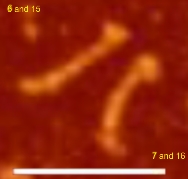
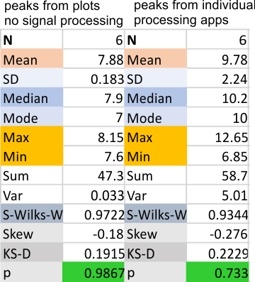
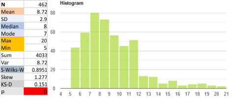
Parallel plots of a trimer of SP-D, AFM and shadowed TEM, took me about three seconds to pick two arms of SP-D, one from an AFM image one from a shadowed TEM image. No problem seeing similarities, the similarities in peaks were immediately apparent and similarities were pretty striking.  Even though shadowed images have that typical lumpy background and it is a little difficult to ‘swallow’ the possibility of there being structural information in from both methodologies, the images confirm the number of peaks in a trimer of SP-D.  i think the evidence which is just an observation here might be substantiated with more samples. The bottom line is that it is very clear that there are many more than the reported 3 peaks along the AFM and the shadowed images. The three known peaks ( N termini junction, glycosylation peak(s) and the CRD peaks).

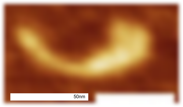
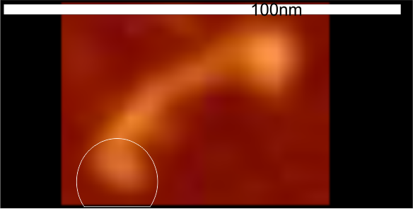
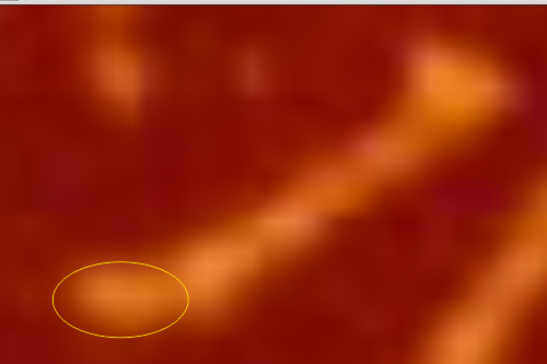
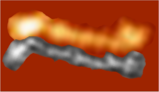
Images were adjusted so that these “cropped out trimers” have the N terminus peak on the left, CRD peak(s) on the right and a grayscale plot was made to compare peak heights widths valleys, and of course peak number. Top image AFM, bottom shadowed TEM.  In the two trimers below the N terminus peak is very bright since I cropped the trimers from dodecamers (where the N term peak is x4 where the four trimers are joined.

The difference between the top AFM image and the bottom that is immediately noticeable  (and confirmed in other plots) is that the trimer in the AFM is glycosylated, so next to the N peak on the left, the bright peak is the glycosylation peak.  The SP-D used for cropping out a trimer for the bottom part (shades of gray) of the shadowed image has not been shown to be glycosylated, so a glycosylation peak is not expected…… therefore that bright spot in the AFM denoting glycosylation is NOT that bright, more like a “low peak” in the gray shadow-cast image. Other peaks along the respective plots are very similar.

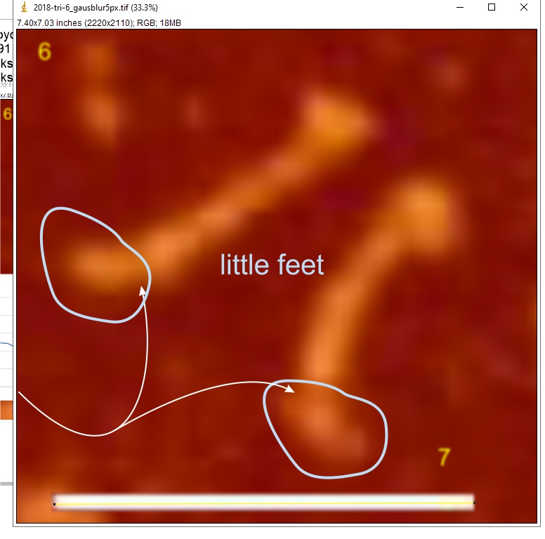
The biggest differences are 1) the tiny peak in the valley between the N term peak and glycosylation peak is prominent in the gray shadow-cast micrograph, 2) there is likely no glycosylation (or minimal) in the SP-D preparation that was shadowed (i have an AFM of that and will compare). 3) See the red circle for glycosylation peak on AFM image and not that bright peak where glycosylation would occur on the shadowed image (dotted line circle). There is a definite “foot” bend in the N term portion of the shadowed image, but also somewhat seen in the AFM image . The plots are very comperable 4) and the low brightness between the N and collagen-like domain is really prominent, and means something important in my opinion.

A new plot and set of images (3 this time) are below.

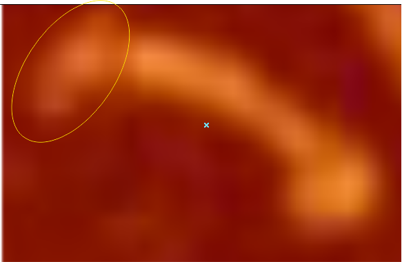
Since the biggest difference between these two arms, besides the methods of imaging, is the peak that is supposed to indicate glycosylation is different in all three.  The top image below is definitely glycosylated (Arroyo et al, 2018) the AFM image at the bottom of the figure below is “possibly” partly glycosylated from the same authors.  There is only ONE image of their deglycosylated SP-D dodecamers that I could find, from which the bottom SP-D trimer was cropped for comparison. The other three arms of that particular dodecamer labeled as deglycosylated SP-D had varying peak heights at the alleged glycosylation site. Whether one, two or three strands of a trimer are glycosylated seems to be an open question, and all the AFM images seem to indicate this since there is consistent peak brightness (height).

The particular trimeric arm of the deglycosylated SP-D molecule (so not a separate trimer, hence the high N term peak brightness), was selected not because of the glycosylation peak absence just because it had similar angles and would fit nicely one above the other. So the orientation was the primary selection bias, not the glycosylation peak height.

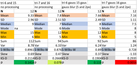
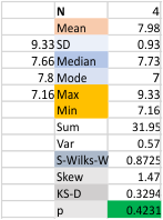
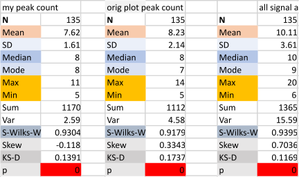
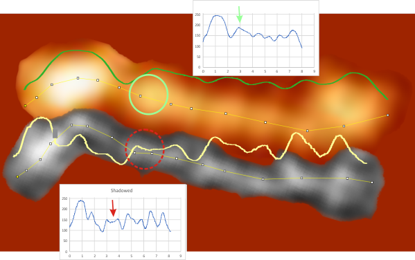
An assembled graphic (below) was prepared with molecules with an approximate shape, size and curvature to show three things: 1) the deepness of the valley between the N term and collagen like domain peaks, 2) the difference in the shadowed image (for which dodecamer the glycosylation state has NOT been determined, but it appears as if it is NOT glycosylated) and 3, the similarities of the peaks (excepting the variable glycosylation peak(s) of the three trimer sections of dodecamers with the two methods, and two separate preparations of SP-D.  The grayscale plots on the right hand side of this image below shows the exact tracelines and the resulting plots for each trimer (obtained in ImageJ, exported to csv, plotted in excel).  The exciting thing is that the peaks in the two prep methods (AFM and shadowed) are just really wonderfully similar.

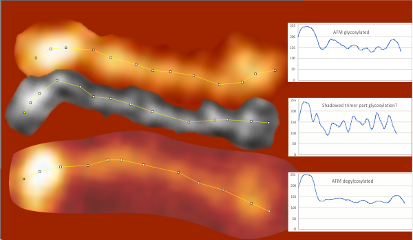
I had been skeptical of cropping out any SP-D arms to trace for grayscale levels in the shadowed image and just gave it a try… lest anyone accuse me of “doctoring” data…. no data have been changed, just the outlines.   AND one really nice results is that the tiny peak that i have mentioned hundreds of times, that lies in the valley between the N terminus peak and the glycosylation peak is prominent in the shadowed image.  If you look at the middle plot left hand side, you see the first tall Nterm peak, and in the shadowed image, a smaller peak on the downslope shoulder.

Little “feet” at the N term side of SP-D trimers

I have looked at these image for years, just now thinking that the bend that is sometimes seen on the N terminus side of the SP-D trimer has an impact on how those multiple N termini junctions might assemble to make multimers with different attributes at that junction: whether end to end, one top the other, or bending for form a ring as is seen more often in multimers with many trimers. So while the flexibility of the CRD regions of a trimer, which are easily seen in AFM image of SP-D are pretty obvious, finding a low spot, a reasonably “thin” part of the molecule seemingly just between the N and collagen-like domains, I have seen on hundreds of plots, however, that it has a “flexibility” is certainly something to think about (per image below).

Two trimers from the same AFM image are shown below, rings are drawn around the “bend”, arrows point to a very low point in the grayscale scan which is a very common feature of SP-D near the N term bright peak.

AFM images of SP-D trimeranother image with an N term “foot” like bend

another trimer with an N term “foot” like bend

…and another one

I looked up all images in Arroyo 2018 and totalling up 50 trimers, only 5 had that little crooked hook at the junction of the N term domain and the collagen-like domain.

Peak number (grayscale plots) in SP-D trimers

19 SP-D trimers (AFM images from several published articles) were counted many different ways to determine peak number. These methods have been described many times in previous posts.  135 plots (129 of which were images that had NOT been filtered, and one image (trimer – 1) which had an additional plot from a gaussian blur (5px)).  The three columns below represent (left) my count of bright peaks directly from the image, (center), my division of the grayscale plot (done in imageJ),  and (right) the 5 signal processing apps applied with consistent functions over the images. The data show “more” peaks found in the signal processing group which also showed a larger standard deviation, also a few more peaks found observing the csv plots, and the fewest (though not significantly fewer than the hand counted peaks from plots) as they are seen in the image. The mode and median from the image and the ImageJ plots are the same. There are differences in each of the signal processing apps, enough so that the peak finding in the whole dataset does not make a normal distribution.
peak detection along a trimer of SP-D
When each of the 5 (plus my counts)=6 peak finding apps were analyzed separately  the difference was seen below.  On the left, my peak determination from grayscale plots obtained from ImageJ, and right, each individual peak finding apps  (the same apps used previously in this blog) applied to each of the 19 trimers, so the total n of plots is still 135, but the n of 6 is the number of different apps used to detect peaks.  The distribution of means and SD from the 6 individual signal processing apps does form a normal distribution.  The difference between the mean of the peaks i count from plots, and the peaks found using signal processing is significant with a 1-tailed t test, (p=.032) but not with a 2 tailed t test (p=0.065).

The next step is to apply image filters to each trimer, and to each of those, apply the signal processing apps to find concensus.  Seems to me that the data will fall inbetween ….  not 7 not 9  but “8” which would be predicted from the similar assessment of dodecamers (plotted as hexamers)… of which I have plotted hundreds and hundreds  (LOL).

I couldnt resist plotting every peak count for these 19 trimers so far…. also, not a normal distribution. The outliers (15 peaks to 21 peaks) all arise from signal processing the plots (yes i could manipulate the functions and make them all 8 peaks, but it seemed to me to be a more honest approach to find a setting and stick with it).  The highest peak counts came from Scipy, and iPeakM80 (Octave). I wonder about the efficacy of changing those parameters to fit my “idea”.