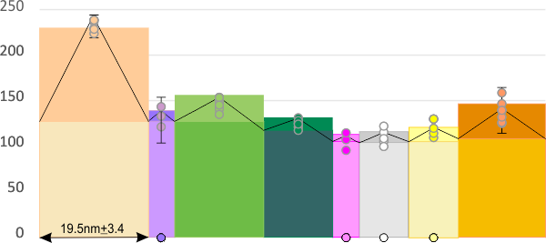
Category Archives: surfactant proteins A and D

PeakValleyDetectionTemplate.xlsx, smooth 11 for peak identification on SP-D trimer

Using the PeakValleyDetectionTemplate.xlsx from Tom O’Haver, I ploted a single SP-D trimer, forward blackward, mirrorred, reversed using excel, as well as bottom to top and reversed.  (PeakValleyDetectionTemplate.xlsx, smooth 11. Peak identification on SP-D trimer shows very little change in peak number, width, height and valley (as determined by grayscale plots made using ImageJ) no matter how I enter the csv file. This is good in a way, as it means the high peaks next to the low peaks, at (smooth 11) pretty much are read the same way, front to back and back to front.

The greater variation comes from image processing and variation in my trace through the center width of the molecule from N term peak to CRD peak(s) at least that seems to be true with this template at smooth 11.

In the graphic below columns on the right hand side are “image” (= my peak count), “plot” (=my peak count from the ImageJ grayscale plot). “peak finding” (= peaks found using signal processing apps – mentioned many times in previous posts). the center row of data for peak numbers is derived JUST from the PVDTxlsx peak numbers.

Rows 3 and 6 are plots of the same trimer using the unprocessed image and gaussian blur (5px) image respectively.

I do think the number of peaks per trimer will turn out to be “8” as these numbers are an n of 1, just to determine whether the peak finding xlsx plots are influenced by direction of the plot line…  The image used for these plots was particularly nice and that would be selection bias toward more peaks.

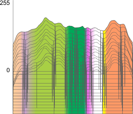
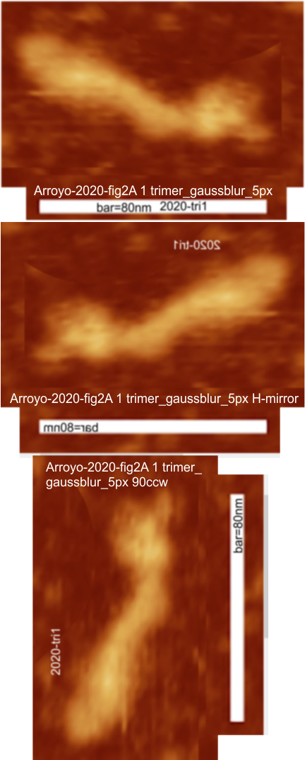
11 peaks found in a single SP-D trimer plotted 14 times, 90o ccw, left to right, right to left, and as a horizontal mirror

11 peaks found in a single SP-D trimer plotted 14 times, 90o ccw, left to right, right to left, and horizontal mirror (see AFM images below).  The plot app was an excel file for finding peaks and valleys (PeakValleyDetectionTemplate.xlsx, the initial traces were done with a segmented line at either 1 or 5px line width using ImageJ.  (Credits for the AFM of the SP-D trimer image, the excel file and imageJ have been given countless times in previous posts).

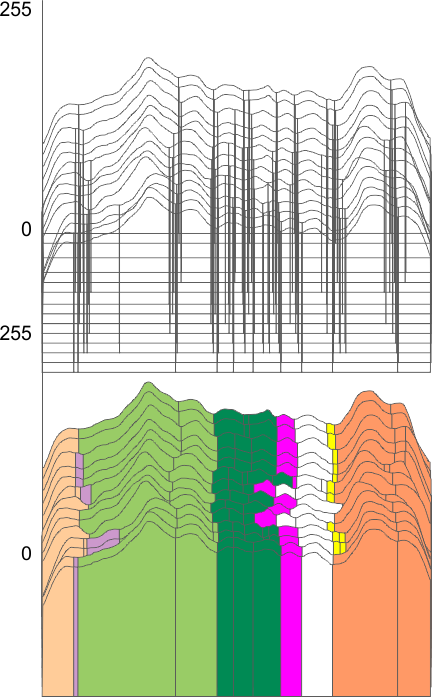
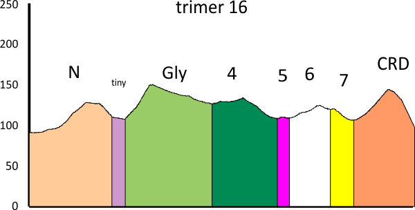
The ridge plot here shows the “alleged 8 peaks in a trimer”(found in previous data from plots of hexamers) as a backdrop to the “actually detected peaks for this single trimer by the PeakValleyDetectionTemplate.xlsx where I tried to use the actual plot lines (and their deviations) as a correlation with what has been seen with previous studies.  N peak on the left; tiny peak=purple; glycosylation peak(s) typically more than one), bright green; peak 4 as yet undescribed with about 3 peaks or ridges, dark green; low and thin peak 5, pink; broad and low peak 6, white; neck domain peak infrequently seen, yellow; CRD domain peak typically multiple peaks (in this image 2 peaks) distinctly large and bright, orange.

It becomes apparent that the concensus peak number for this single SP-D trimer is 11 (top ridge plot). My designations for why peaks could be sorted “down to 8 peaks” was  made on the basis of hundreds of plots of hexamers (within dodecamers) where concensus was 15 peaks per hexamer, This creates trimers with 8 peaks, the N term peak being blended in higher order multimers.

The divisions of the colors from the actual plots (two of which I should obviously re-sort in retrospect but were made looking at the plots at the time they were traced (these being the dark green, pink, white columns aka peaks 4, 5 and 6 in the fifth and eighth plots up from the bottom).


9 plots compared for SP-D trimer peak number

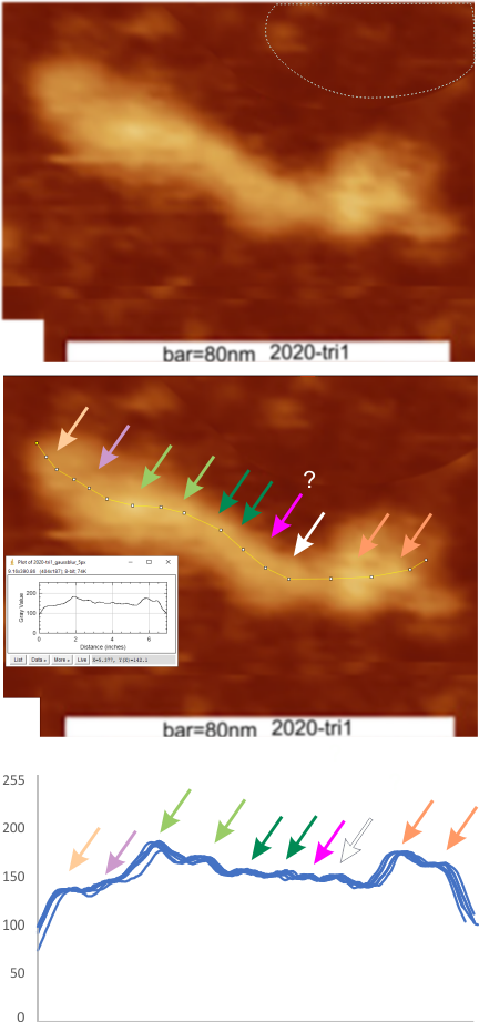
A single image (from Arroyo et al, 2020, that I named trimer 1) with bar marker and nm value was plotted nine times. This means tracings right to left, in original images and images mirrorred and image rotated 90 ccw. These plots were traced in ImageJ opened in excel without adjustments (so the x and y values were not changed) and the multi-blue-line plot at the bottom of the graphic below is the result of superimposition without any editing. The plots are virtually identical. The peaks counted from individual plots was 10.5 peaks, ranging from 9 to 12, there was no mode. The top image is the original image, screen printed from the publication. The dotted line in the upper right is where I cut and pasted background over an identifier in the original publication (just to clean up the image). The image was filtered with a gaussian blur of 5 px.

Some of the tracings were made with a 1 px line, and others a 5 px line.  There are slight differences, but 1 px line was chosen for hundreds and hundreds of tracings in this study.

The image of the trimer just below is an example of the tracing, which I began at about a medium grayscale into the molecule and ended similarly at the other end of the molecule. The tracings varied from right to left, and right to left and each plot was also transformed in excel when applying peak finding.  Plots were mirrored so that the N term is on the left, the “tiny” peak and the large glycosylation peak(s) are next.  As yet unidentified peaks have arrows pointing to them, and where peaks were detected in the plots but not by “eye” i put a question mark. The two peaks on the right are the CRD peak(s).  I have kept colors of peak identifiers consistent throughout all the posts in the last two years, so previous blog entries can be compared.  I am convinced that little variation exists in the way I execute these tracings, or in the way (direction, mirrorred or rotated) ImageJ processes them.


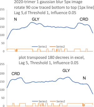
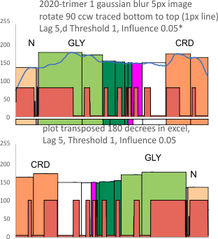
Reverse? plot peak detection

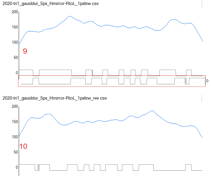
I am not sure why the transposed excel column (first line becomes last line) was plotted like this in the stackoverflow app for peak finding. ?  The rows were mirrored vertically in excel, but i didn’t expect the peak widths to be mirrored when i plotted the transposed data into the stackoverflow peak finding app.  (see red box below the original excel plot. I cut ans pasted the bottom part of the reversed rows just below the peak detecting series in the top plot (RED BOX).  something very un”right” here.  Suggestions are welcome.

It seems to me that the height of the tallest glycosylation peak when plotted at the end of the tracing influences the detection of the smaller N term peak on the trimer.   Plotting a trimer within a dodecamer (which makes the N term peak about the tallest peak on the tracing, there is the possibility that after passing that peak the influence on the detection of the tiny peak and glycosylation peak has changed.  I think looking at the left and right trimers in a dodecamer this could be uncovered.  I actually think i did that early on.  So on the plot reversed, peak width and height of the glycosylation peak  influences the rest of the tracing.

Using 8 similarly collected tracings 1px thick line and 5px thick line plotted in ImageJ,  of SP-D, with images mirrorred and rotated,  then peaks counted in the LagThresholdInfluence mode from stackoverflow, the mean peak count in a this particular trimer is 10.5, all values appear twice, no mode, however if the forward tracings (that is from N to CRD, peak number is counted it is 10 (min=9 max=12), while if the reversed data is plotted the mean is 10.75 (min=10 max=12)  maybe not an important difference.

This is an assessment of a single peak finding funcion….in addition  I have used Octave’s iPeakM80,  and AFPPxy, Scipy Peak Finding,  PeakValleyDetectionTemplate.xlsx, and my own two non-signal processed assessments, one from the image itself, the other from the plot generated by ImageJ (that plot used by all other functions).

I compared the use of a five px line to trace the moleule, and a 1 px line. I am revisiting that choice but it seems that the 1 px line works fine.

RCSB (as of march 2 2024) still doest not give a full structure for a surfactant protein D trimer (nor did i see hexamers, dodecamers). This means to me that the collagen like domain and the N term junctions are still not really known, in terms of 3D structure…. thus, as has been for years, when one looks up SP-D they just see the neck domain and the CRD domains…

Varying the trace and the direction of “peak finding”, may change the peak count in trimers of SP-D

Varying the trace, may change the number of peaks, and whether this is relevant or whether sheer number of plots of peaks (grayscale 0-255) along a trace of a surfactant protein D trimer (or hexamer) negates these small differences.
There are many ways for peak numbers to change, 1) noted above, the way the segmented line is traced in the AFM images of SP-D, 2) the image processing filters, enhancing or reducing peak brightness, blurs, median and limit range filters, and 3) the specific values for each filter applied in peak finding programs.
I have examined one trimer plot, mirrored and rotated, with separate traces, and each of those transposed 180o in excel and reapplied peak finding programs.
There is some variation, yes, but pretty small, not the big changes like i expected to see. Plots below are a sample comparisons of how peaks are detected in a “stackoverflow” method for peak detecting.

top image shows the plots, bottom image shows how the plots have been ordered (according to countless plots determining that the peak number in a hexamer is about  15, and in a hexamer half that, except for the fact that the N term peak number does change.  That is something that will be interesting to figure out.  Changes are small…  but my purpose was to see whether the “tiny peak” on the slope of the N term peak would be more prominently identified if plots did not have the large N term peak just prior. That has worried me for a long time….. that tiny peak is clearly there but rarely counted.  (it is marked by purple below). The reversal of this plot did not change the detection of the “tiny” peak.

Me vs Peak Valley Detection Template xlsx

There are many things i dont understand about peak and valley detection using functions.

I would have to test out whether the lag and amplitude and influence of the detection works against having a tiny peak detected next to a high peak by plotting this same trimer of surfactant protein D up, down, rotated and mirrorred to figure out how to have it see what I see: that would be to include a tiny peak before the glycosylation peak, and eliminate a much less obvious peak in the middle of the series of peaks that follow the glycosylation peak. I know these things can be selected and I can choose whether to change the parameters.  I am trying to eliminate not induce bias. I like the first lines by this blogger, yes i agree, the human mind is very unique.

This is a real handicap to detection of relevant grayscale peaks in a plot of the length of SP-D trimers. I could of course change the smoothing and other factors but then I end up with a rediculous number of peaks and it no longer is relevant.
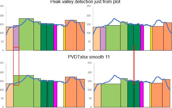
Case in point… plots from ImageJ that I selected peaks on (which are in line with the vast number of plots from which a mean number of peaks along each trimer was established. (peaks on the left, valleys on the right, top row of plots) versus what i find with smooth 11 using (what i think is one of the best peak and valley finding templates around (easy to use, output can be edited like any excel plot as opposed to those that come out of octave functions for finding peaks which are, as vector illustrations, total nighmares to work with). The bottom set is what I get from PeakValleyDetectionTemplate.xlsx offered by Tom O’Haver – thank you). The trimer plotted is from an image by Raquel Arroyo et al – thank you).
The plots are virtually identical in peak number, width, height and valley EXCEPT for the two tiny peaks, one lost and one added.

AFM: one limitation affecting peak number of SP-D dodecamers

AFM: one limitation affecting peak number of SP-D dodecamers, could be what I found on a website. “Due to the nature of AFM probes, they cannot normally measure steep walls or overhangs“. This quote is from a website that is mostly in chinese so I didnt bother to read or translate. BUT it is clearly what I have seen as I search for peak number in SP-D molecules (whether trimers, hexamers dodecamers, or higher order multimers).

Case in point is how many times the “tiny peak” which I have noted dozens and dozens of times as a small in height, narrow peak right near the base of the N term peak. It seems to be missed a lot of the time, there are other times when it is very obvious. A couple reasons for its intermittent appearance in AFM could actually be because of the very steep wall on the downslope of the N term peak before the glycosylation peak.

In terms of “overhang” this might also apply to the blending and disappearance of the neck area which is sometimes covered in the CRD peaks which flop around visibly lying over the neck domain.

Surfactant protein D, peak plots from AFM images

Last couple months I have been plotting individual trimers of SP-D to determine if number of peaks, peak heights, a valleys using the same 6 methods used on dodecamers produces the same results. The same 6 functions were use on trimers as on dodecamers (See list of image and signal processing functions used — at the end of this post).

There is clearly a smaller N term peak (N) in the trimers than the dodecamers where four N term peaks are “piled” or “linked” together. Other peaks do not change much, which is a good thing.

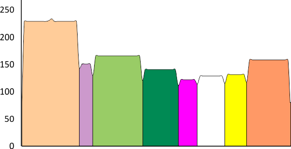
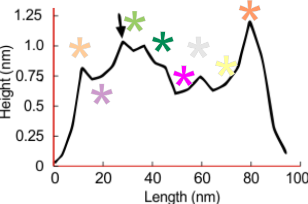
The plot immediately below shows just the peaks plotted for just one trimer (kind of a perfect one), and immediately below that plot shows mean peak height, width, and variation for 6 dodecamers (24 trimers, 368 trimer plots),  and the third plot down is 14 dodecamers (56 trimers, 897 trimer plots) and the line graph below that is the plot from Arroyo et al, 2018 in which she identifies the N peak (peachie orange), the Gly peak (light green), and the CRD peak (orange) ONLY. My purpose was to show that there are at least 8 prominent, consistenly found peaks per trimer, not just three.

So many different images analyzed from different publications with Arroyo as author, are shown, ploted as dodecamers (6 or 14 individual dodecamers) or single trimer, there seem to be 8 peaks per trimer. Widest peaks are indeed the N, Gly and CRD, next widest and most consistend are peaks 4 and 6, the yellow peak (coiled coil neck domain) is infrequent, and during preparation for AFM is typically covered by the CRD domains flopping around, and also infrequent are the small peak called “tiny” because it is both thin and low (but consistently on the down slope of the N term peak) and peak 4 which is broad and rolling like the GLy peak, and a low and thin peak (pink), and a broad low peak before the coiled coil neck.

So after more than a thousand plots, I think I am pretty sure these peaks are part of the molecule and can perhaps contribute to creating a complete protein model of SP-D (which do date has not been done).

https://imagej.nih.gov/ij/
https://terpconnect.umd.edu/~toh/spectrum/PeakFindingandMeasurement.htm#ipeak
https://terpconnect.umd.edu/~toh/spectrum/PeakFindingandMeasurement.htm#findpeaksx
https://terpconnect.umd.edu/~toh/spectrum/PeakFindingandMeasurement.htm#Spreadsheet (s)
https://docs.scipy.org/doc/scipy/reference/generated/scipy.signal.find_peaks.html
https://stackoverflow.com/questions/22583391/peak-signal-detection-in-realtime-timeseries-data/22640362#22640362 (version: 2020-11-08)

Peak finding functions

Peak finding functions are certainly not the end all and be all of assessing peaks in AFM images of surfactant protein D. I am totally disappointed in how they work.  It is so clear that depending upon measures that have preceeded a peak and how big a peak is has LITTLE at all to do with what nature does with proteins (specifically, irregularly placed bumps and twists of varying sizes that can be seen by eye with electron microscopy and AFM and other microscopic media). Not a single peak finding function that I have found has any real comparison to what a trained eye can find (at least at this time). Since the user determines the robotic approach, peaks can vary from 4 to 40 when the eye can see about 15 in a dodecamer regularly.

When I see the divisions of peaks, the numbered peaks, the missed peaks that signal processing produces i think to myself. Why that, or why not this.

Sadly this makes everything I have tried to figure out about unbiased counting, height, width and valley depths, using image processing and peak finding, in surfactant protein D trimers (and dodecamers) is pretty much NOT verifying anything except the fact that they dont work.

Being adaptable mentally just is still a human trait……. how much longer, I dont know. Training seems still to lag behind human abilities.

Things I have noticed:

1– in the trimers, it appears that multiple peaks clustered (maybe 2 or 3) seem to happen when there are (as in the case of the glycosylation site (published data) the three trimers at the glycosylation site have shallow staggered peaks, as if there is a rotary positioning. Seems logical that the lumpy effect would be found when rotating a repeating event (like glycosylation).
2– signal processing functions are not very adaptable, they do not see pattern well, they ignore some peaks and find others in a way that is inflexible

3– N term peak height in the dodecamers and higher multimers shows variation in N term attachments.