

Category Archives: Methods to assess TEM and AFM images
Four dodecamers: N term junction peak valleys
The peak height has been found, the valleys on the side of each peak progressing to the center (inward sid of the peak, coming from the CRD toward the center, thus the right hand side of the left part of the image, and the left hand valley side coming from the right CRD meeting in the center where the N term peak is.
This means that each trimer valley value is taken from the side directed toward the N term peak As recorded for widths and peak heights, the valley height is measure in all the separate trimers (N=172)(N=4).

Four dodecamers: Peaks 6 and 7 height and CRD height – grayscale 0-255
Plots of SP-D trimers (as hexamers) with the N term peak becoming a whole peak (not just a half peak as the molecule would suggest happens..this done for ease of calculating thus each shows 15 peaks per hexamer (an odd number) or 8 peaks per trimer. Using many plots ( grayscale plots obtained in ImageJ), peak heights are being determined for each peak set, and these data are for peak 6, as yet unnamed but present at least 90% of the time in this dataset — 100% of the time in the plots for two molecules, 95% in one molecule, and 82.5% in another). Using just the summaries for the four dodecamers (without the missing values) the peak height for peak 6 is 115+/2.6 Screen prints from excel are below.


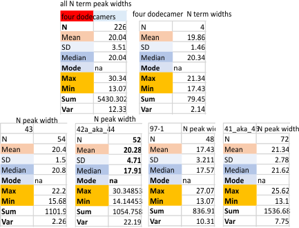
Four dodecamers of surfactant protein D, replicate N peak width
Four dodecamers of surfactant protein D, replicate N peak width.
Previoius values for the width of the center N termini junction of surfactant protein D dodecamers (from AFM images published by Arroyo et al), comprised a large dataset, hundreds of plots, four different dodecamers and the means for N termini peak width and all the other peaks (8 per trimer) were posted as well. In this new dataset, the Gwyddion processed images were not used because of the huge differences in grayscale values (Gwyddion exports as R, not RGB, and I assume that is the reason – at least I could not figure out how to export images processed in Gwyddion as RGB). Some plots were used in both datasets.
Also, the very far out image processing filters were eliminated, and the new set really is focused on 5 and 10 px gaussian blurs, very little else. ( i can make a list if someone would like it). Also, instead of hundreds of plots, there are many fewer, but very surprisingly the data from the big set of grayscale plots, and this abbreviated set are so close, that I think there is no reason to plot and process every image in all permutations and combinations of signal and image processing.
Comparisons are below…. listed as old and new, for the whole column – for the individual dodecamers (listed by name as 41_aka_45, 42a_aka_44, 43, and 97-1 — designations only for record keeping), and again, with an N of 4, using the N termini width for each dodecamer individually.
The n for the N termini peak width values duplicated…. a complete N width for each trimer, so the actual n is “half” that (see the (/2) notation on the excel images.


Consistent approach to saving images used for image and signal processing in microscopy?
I wish I had known how much work I created for myself by using images from different programs, different ppi, different RGB, CMYK, grayscale, and dimensions. A little standardization in my approach would have made getting the data much easier. A word to the “wise”.
My images were from so many sources, so many were pixelated, low contrast, warped, screenshots from publications, and general inconsistent in quality, and made by different microscopes, and different microscopic techniques. A polyglot for sure.
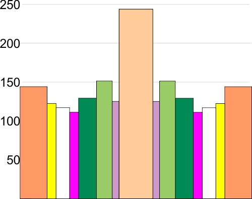
Four dodecamers of SP-D, summary of peak number, peak height and peak width for 300 hexamers
Here is a plot of the height and width (summary of 600 different plots of SP-D trimers)
I have sorted the plots by hand into the “mean number of peaks per hexamer that was found for this same dataset” So you see 15 peaks, you see the fifteen divided (mirror on either side of the N term peak (peach), tiny peak on the downslope of the N term (purple), peak =glycocylation peak (medium green), peak 4, unknown peak, large, and also wide (dark green), unknown small peak (peak 5, pink ), unknown low and broad peak 6, (white), and peak 7 likely the neck domain of the hexamer (yellow), and peak 8 the CRD (orange). This is the a mirror (n=300 plots) of the left and righ trimers (n=600). X axis is percent of width, Y axis is grayscale value 0-255.
The images exported from gwyddion were not included in this dataset because of the huge difference in the grayscale values for images exported R vs RGB when plotted in ImageJ).
Peaks within each of those peaks is shown here. The peaks which are not present all the time have a value less than 1, those with a value of more than one often have more than one peak as sorted above. List is for a trimer…. begin in the middle of the above graph, and move to the right (and mirror to the left from the N term peak). This means that a minimum, there are five consistent (not the published three) but five peaks found all the time. That is the widths… peak 1 (N terminal domain 26nm), peak 2, unknown peak (3nm), peak 3 (glycosylation peak 10 nm), peak 4 (undetermined function, 12nm), peak 5, undetermined function (4nm), peak 6 (undetermined function 7nm), peak 7 (likely the neck domain that sometimes is seen sometimes covered by the CRD (4nm) and peak 8 (carbohydrate recognition domain (12nm).However, I am doing more valley determinations to provide a “background” or “baseline” for the peaks which will likely NOT be a straight line and may give information on the “slope” of peaks.
Images processed with limit range filter — and resulting grayscale values
I am pretty sure this is just because exports from gwyddion are the R of RGB images, any help coming from the community that uses Gwyddion is welcome. It causes some problems when using ImageJ plots of the gwyddion exported images and images exported from other image processing programs (as in every other program i have tried (about a dozen).
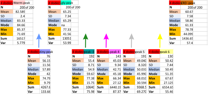
I found the peak heights using just the images processed with gwyddion, in particular the limitrange filter as a separate data set. Results are below. It is clear that the three peaks which have been published (N, Gly, CRD) per trimer are present 100% of the time (in this case, all 200 of the 200 trimer plots. There are two other peaks (peaks 3 and 5 which occur because of their characteristic shapes…. they were easy to recognize. That is peak 3 which was at least a broad as the glycosylation peak, but usually lower peak height, and the broad flattened peak (peak 5) also low on the grayscale. These were present about 95% of the time. The peak that sometimes shows up (most likely the coiled coil neck peak is peak 6 and depending upon the position of the CRD, it shows up, or doesnt show up (likely covered by the ability of the CRD domains to land in different positions during processing. CRD does appear as one, two or three separate bright areas at the C-term end of each trimer. This also makes it a “choice” where to draw the segmented line that becomes the grayscale plot in ImageJ.
These data are for images processed in Gwyddion, and peak numbers (see previous posts) are determined mostly in several signal processing programs (Octave, PeakValleyDetectionTemplate xslx, a LagThresholdInfluence plotting algorithm, and scipy peak detection algorithm).
Sorting peaks into the peak numbered from N (peak-1), tiny peak (peak-2), glycosylation-peak (peak-3), unknown peaks, 4,5, likely neck region (peak-6) and carbohydrate recognition domain (CRD peak 7) is done manually.
Means and other values prepresent grayscale (0-255). Three highest peaks (top row of values) are those that have been consistently reported in the literature. Potentially additional peaks are the 5 boxes below.
Getting closer to making a “concensus SP-D LUT plot” from which to build an AI model
Getting closer to making a “concensus SP-D LUT plot” from which to build an AI model.
I had four SP-D dodecamers to work with, literally hundreds of plots, 5 different plot peak finding algorithms (apps, programs, websites), and a dozen different image processing programs, all to find the perfect peak plot for SP-D hexamers. These molecules are bilaterally symmetrical (three identical x three identical) with the N term junction in the center. Little is known about the central connections though the CRD and neck regions have molecular models. Taken about 3 years to try to figure this out, input would have been (would still be) very valuable.
I am hopeful that an easy technique will be the outcome, that is an easy technique for assessing peaks in many different types of molecules (images from AFM at this point), particularly those which are bilaterally symmetrical.
Four dodecamers: peak(s) 8 width – carbohydrate recognition domain
THis peak has the closest to registering two peak(s) within the larger element of a whole CRD peak area.

THis peak width (just under 17 nm is close to what has been seen before.
Number of peaks within the CRD whole peak depends clearly upon the path of the segmented line used to trace that end of the SP-D trimer.

Four surfactant protein D dodecamers: N termini peak widths
Summary of peak widths (valley to valley) using image processing as well as five signal processing programs to calculate that dimension. In one sense the results are really good, in another sense they are basically so similar to those just done by “my minds eye and a good measuring stick” that the two years has provided no new information. 20 nm is a very stable number for the valley to valley measurement of the N termini junction of surfactant protein D as is shown in AFM image. This value is found as all trimers with the full N term peak, as for each of the individual molecules that have been measured (in this case my numbers for them are arbitrary: 41_aka_45; 42a_aka_44; 43; and 97-1) and also the mean of the four dodecamers (N=4) . The number of trimers measured in one molecule was greater than the other three so this data set was primarily made only those plots which have similar processing. That is with 1: images with no processing, 2: images with a gaussian blur (either 5 or 10px); images that have a gaussian blur and a limitrange filter. 3: each of those images from each of those groups of image processing were then exposed to signal processing by five different algorithms (as part of several programs: Octave (Autofindpeaks.m, and iPeak.m; Scipy; LagThresholdInfluence (batch processing) and an excel template for Peakand ValleyDetectionTemplate.xlsx). Therefore the balance of bias was similar among the four images of SP-D.
 The tiny peaks on either side near the valley of the N term peak are located by image and by a combination of image and signal processing algorithms only about 31% of the time. This is a little disappointing, but hand counting the peaks provides a more robust counting of those tiny but very consistently found peaks.
The number of peaks WITHIN the N term peak varies from 1-2 typically. About 50% of the N term peaks consist of two identifiable sub-peaks. The widths of the sub-peaks is not always equal and depends upon how the segmented line is drawn through the image.

Width of the peaks is about 3nm wide, which still can be identified within the micrographs very often. In this set there is one value which is large, skewing the data. 
I calculated that single image without the large value below.
 Here is the information (peak width in nm of the tiny peak) from months and months ago, which literally has not changed with the addition of the signal processing assessments. I dont know whether to be happy this didn’t change, or be miffed because of the amount of time to confirm that the original assessment was pretty good. Tiny peaks appear about 30% of the time (rather are measured as “peaks” by the five signal processing and one image processing plots about 30% of the time. There are many times that tiny peaks are visible, just are not counted.
)