My worksite for my newest concrete pot outdoor scrap-mosaic creation is as messy as any creative art-site could be. Just stones, jewels, tile, junk, spacers, dirty rags, water, trowel, sand, ants-bugs, and dirt everywhere. I think the rush comes from sitting in chaos trying to create order from that which is a temporary mix of chaos and order so that if just enough order is actualized, just enough to fool people into thinking there IS actually order in the universe while there really is none. (LOL)
Monthly Archives: June 2019
N termini of SP-D and side to side arrangement?
This is what I think SP-D fuzzyball arrangement looks like. I wonder if there is the possibility that there is N terminus binding more similar to SP-A and MBP, the lateral associations (as well as a hairpin turn between two trimers of SP-D to form a fuzzyball with a “hollow” (more or less) center as seen in many images. Two images here from a 14 armed-fuzzyball of SP-D (image not mine originally but highly processed for showing the N termini, the collagen-like peaks that occur along the arms and the possible neck and then the prominent CRD domains. It is a thought…. you are free to criticize and discuss… but this is a visual assessment only, i have no data except three years of “looking” as confirmation.
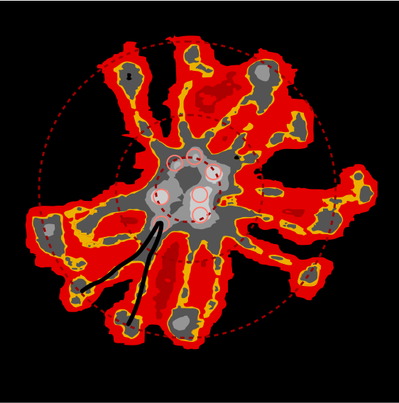

Center of SP-D multimer
The N termini of a multimer of SP-D still seems to me to be a “ring” rather than a center bundle. The ring in the case of this image (not mine) measures about 20 nm in diameter and each of the arms about 40 nm. These measurements are relative to concensus measurements on SP-D (typically the dodecamers) and I am not at all convinced that most individuals use correct micron bar markers. In fact, in images where fuzzyballs (SP-D multimers) appear along side of dodecamers, I wager that they are slightly more compact, per this image from Hartshorn et al (Respiratory Research, 2008) keeping in mind that this particular SP-D is a mutant which they label as Met11, Ala160, their bar markers and image below. Diameter of a dodecamer is actually 130 nm according to their measure (which is in orange, at 100 nm). There is no center gap in this particular multimer, however there are also many many arms and the center ring might actually be shown here dimensionally covering what would be a center dark area as seen in multimers with fewer arms. 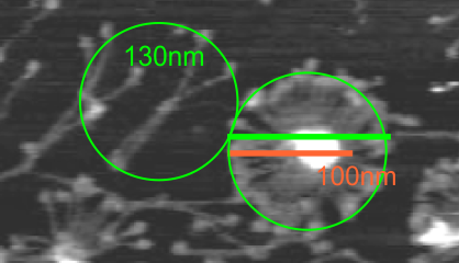
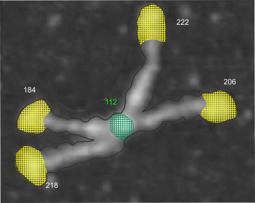
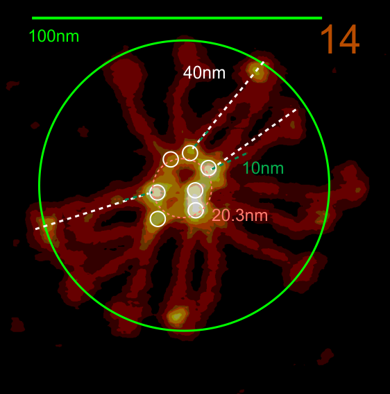
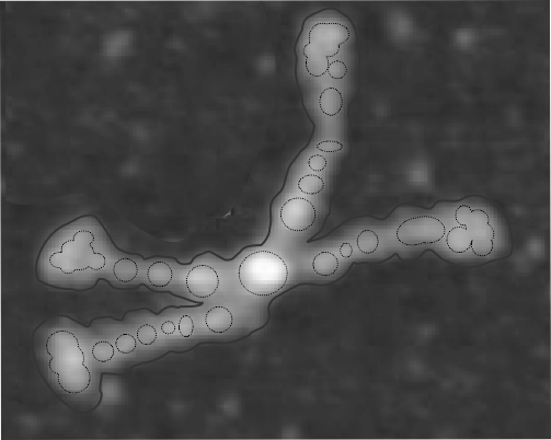
Here is another AFM (not my image) which shows the center ring to be about 20nm in diameter, and each of the arms of this multimer (three measured here) measure at about 40nm. The main peak lateral (circumferential) to the Nterminus peak in dodecamers which lies in the collagen domain, is about 11nm in width, (as seen on many previous posts for dodecamers, on this blog about SP-D) and is also measures about that in this image… in terms of distance to the peak of the Nterminus. I take this to mean that the center of the multimer is NOT at the center of the whole molecule… because it is just NOT a peak, but a valley, but instead at the center of each of the bright dots (in this case 7 bright spots in a ring of this SP-D multimer of 14 arms).
Not so clever an approach, but a pretty picture of SP-D
Just cannot figure out how best to narrow down the dimensions of these images. But this one is kind of interesting, and the grid (at nm2) makes a nice place for conversion to 4 or 5 levels of grayscale, and provides a measure of x,y and z in sqnm.
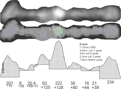
LUT (grayscale) 3D plot of SP-D (two arms of a dodecamer) Peaks – not valleys
I manually changed the values from 0-255 on each of the pixel determinations that I retrieved from photoshop (previous post) to make these peaks not valleys.
Original AFM image (one of the two double arms of a dodecamer – CRDs on each end N terminus in middle) on top, sliced and diced and straightened and exported image for Photoshop and pixel determination (which determines – more or less_ the width of the various regions of the SP-D arms, and 3D plot then in excel. and plot from ImageJ, and measurements in NM and grayscale (labeled here luminance – which it probably should not be called).
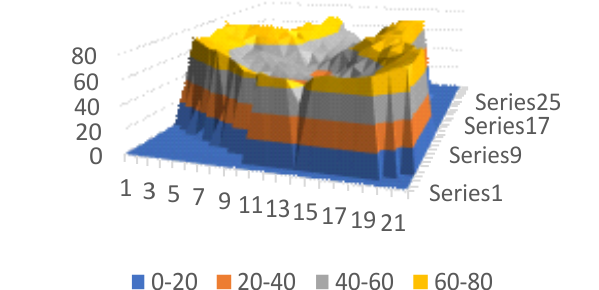
LUT (grayscale) 3D plot of SP-D (two arms of a dodecamer)
 easy to see the CRD, the N terminus where two trimers join in the center (looks like a blue lake) (peaks are “valleys” here so I need to do something about that). The peaks at the junction of the collagen-like domains and the N termini are the next highest (lowest here) peaks (orange).
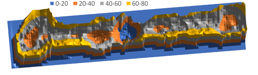
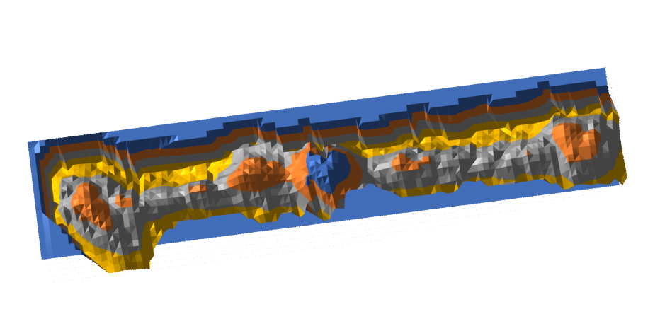
Simpleton inversion (shadows are important in graphics) makes these peaks.
Half an arm of SP-D dodecamer 3D LUT plot
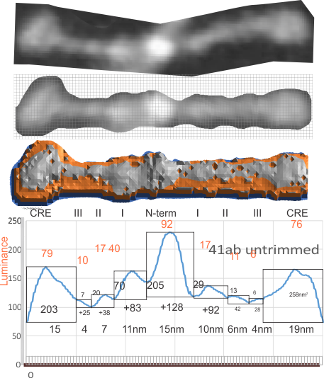
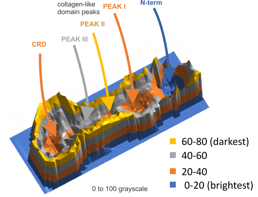 Having fun with this. It does show the width of the AFM micrographs better than taking just a single line or a thin rectangular plot of a straightened SP-D dodecamer arm. I like the way the obvious thinning of the height measures work over the collagen like domain peaks, as well as the spread of the trimers where the CRD sort of fan out. The collagen-like-domain (labeled peak I is not only the tallest of those three peaks, but the broadest as well and may include part of the coiled coil neck? Any comments are welcome. The N terminus peak is on the right hand side, and has a value very close to 100% in this grayscale plot (using photoshop picker tool at 1 nm2 intervals (thousands of them) and excel to plot the image. It should be reversed (100 – 0) to make the image inverted. This goes further than the blog yesterday which was just really the CRD.
How to use LUT tables in a 3D plot for arms of SP-D dodecamers?
Painstakingly – slow, getting the grayscale values for each nmsq. Here is a plot for just the CRD for one arm of a dodecamer of SP-D. I will see how it turns out and whether it will be rotatable and altered to look more like it should. I don’t know how to export this as a vector file yet. The image should be inverted (not flipped vertically… but color inverted) so that is a problem as well.
More on RGB to grayscale conversion of AFM images of SP-D
Another post giving the math for converting RGB to greyscale is found here.
It seems that Luminosity, Lightness and Averaging are three methods which are used often. I am looking for someone who can find which of these three methods Photoshop 6 and CorelDRAW x5 uses to convert RGB to greyscale. (CorelDRAW under “autoadjust” and
In photoshop 6, thresholding a black and white image just doesn’t really help (in my opinion) because there is too much loss of the greys.Below is an image (used many times before) of SP-D (not my AFM images, someone elses available online) which I have manipulated in photoshop using image/adjust/levels, and image/adjust/autolevels, and image/adjust/autocontrast, and image/adjust/contrast in various ways. I will plot my favorite arm (upper left) which has three peaks between the N terminus center high point and the CRD, having probably appeared more times than any other configuration, and the pic is also biased to my assumption from previous LUT plots, to have three different heights for those three peaks, and also different widths. I will post plots in for that same arm, in the same order below. Top left, image as used previously (test 1) provides a great plot.
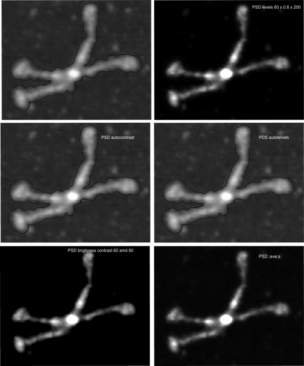
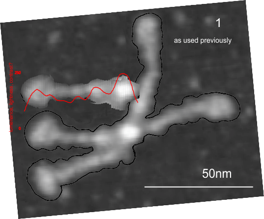
Test 1, image as used previously, not very much adjusted (i cant remember but likely some contrast increased and brightness reduced after the original conversion from color) but done in the same manner as other SP-D dodecamers that have LUT plots (see countless previous posts).
Confirming, and reconfirming previous LUT plots, there is an N terminus peak, three intermediate peaks (in this case the third peak from the N terminus is pretty small) and the bumpy peak of CRD (owing to its distribution of the three CRD domains in a large bulb like end.
Little adjustments, same peak, so that points to the small effect that the several different algorithms for changing RGB to greyscale may not matter as much as I thought. Here is a link to another article on converting color to greyscale. and yet another on terminology and greyscale (ok, so i need to remember to use grayscale not greyscale) conversion.
 While i know to little about this to have an opinion, my basic understanding is that most of the conversion software attempts to mimic what the human ee sees, rather than wht the RGB actually convert to.. in terms of — Gray = (Red + Green + Blue) / 3 — which for science, i.e. looking over micrographs) probably needs to be as free of attempts to increase or decrease the “RGB” values to fit human perception. SO, that said. perhaps less manipulations, fewer algorithms might be the best approach.
I have used RGB conversion in photoshop, in coreldraw, and desaturation to convert RGB to grayscale (yep now gray with an “a”).
After reading (rather stumbling through) some manuscripts and blogs about dozens of RGB to grayscale equations … my decision is to go back to basic grayscale = R+G+B/3 rather than use all the fancy formulas that make the grayscale look more pleasing to the human eye and automatically adjusting the blue and greens to make things look “nice”. Then I can adjust the contrast to what pleases my eye, emphasizes what I am looking for, and brings out the structural detail in my images, manually, and define it as such. To find the codes that were used in some programs is totally impossible, and if found are probably just as biased a conversion effected by my “hand made manipulation” of the images. If the conversion from RGB to grayscale is standard and the adjustments, tweeks are mine I can just comment on them in a line of text in the materials and methods… ha ha
Who knew that was (could be) so complicated. Hahaha…
FOR ME…. my eye is still the best tool to convert and desaturate and change the brightness and contrast. It might very well be biased, but at least it is not brainless.
Here is the SP-D dodecamer I see
It is easy to see that there is a definite width variation in at least three different places. Center N terminus peak is not the widest, though it is the tallest “Lightness” or “luminance” peak. The CRD (four outside areas are the largest in terms of width, but not the tallest but next tallest and it is the greatest in square nm (in this image, each being about 200 nm2 while the N terminus is about 100 nm2). I guess at some point someone needs to do area under the curves for both width and height and get a total nm for each of the regions. It seems that there are three peaks and also a little blip for the area just before the CRD (presumably the coiled coil neck region, that means four peaks between the N terminus and CRD. And sometimes it looks like 5.
Nm grid overlying area of the N terminus and CRD shown below. The nm of the largest peak between (and next to N terminus) and CRD is something about half the size of the N terminus nm2.