What I have experienced in 55 years of microscopy is that I like what my eyes see (with my mind’s eye) better than I like what i can “quantify” using the tools currently at my disposal to tell me whether what I see is significant or not.

In times past, the tissues were logged with numbers (after 100,000 blocks I certainly could not remember a number and animal treatment group) the sections, slides, the grids, the stains and the order presented were kept “blind”.  The data were talled according to the random choice of image in a random choice of slides or grids examined, all in an heroic attempt NOT to be biased.  And why?  Bias is easy to insert. Unknowingly inserting bias leads to significant error in science.  Bias is inserted both “for and against” the predicted results, and either direction damages the credibility of the data.

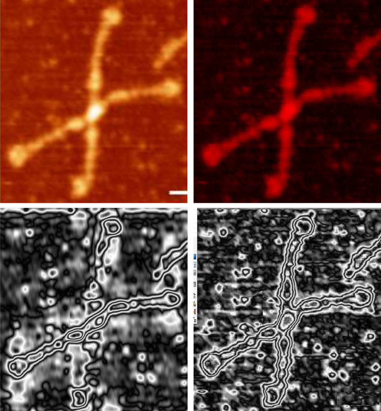
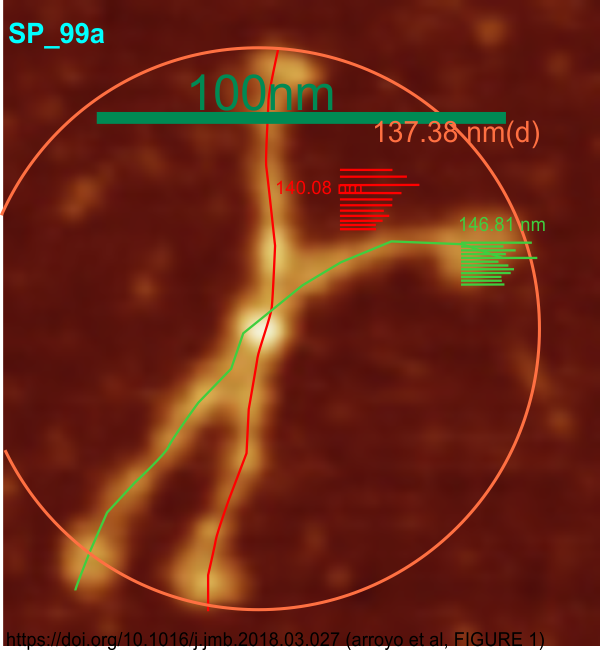
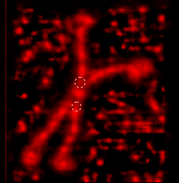
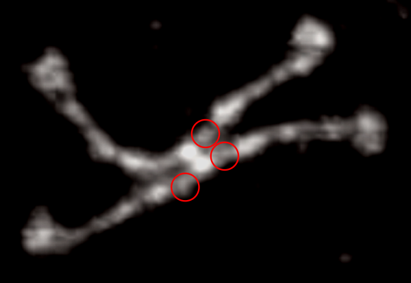
Some stereologic and morpometric methods I have used, invented for a particular purpose where no such method was previously described.  It became a test of my ability to see variations in tissue whether methods I devised could ferret out what I “thought” I could see.  If i saw a change, altered structure, greater or lesser incidence, odd shape or position after going through my slides or grids, I devised a way to acquire enough data points to decide if the change was significant. Rarely did anything I perceived as altered structure turn out to be chance…. — and could usually be sorted into an experimental group quite easily. Without going into examples (of which I could relate dozens) this is the dilemma for surfactant protein D.  I have no doubt in my mind that there are between 4 and 6 “luminance” peaks between the N termini and the CRD for each of the trimeric arms.

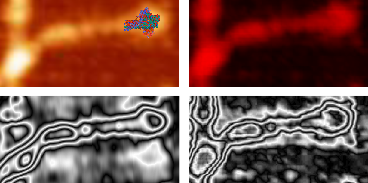
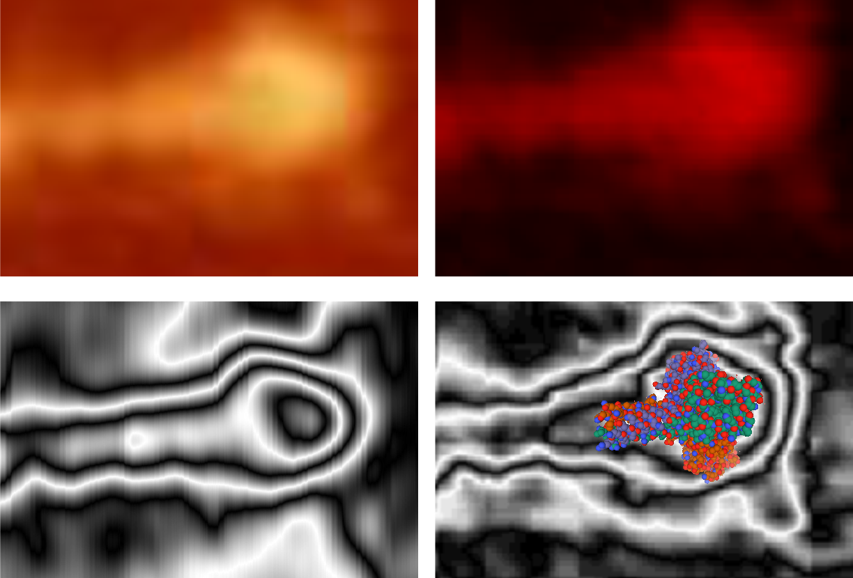
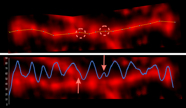
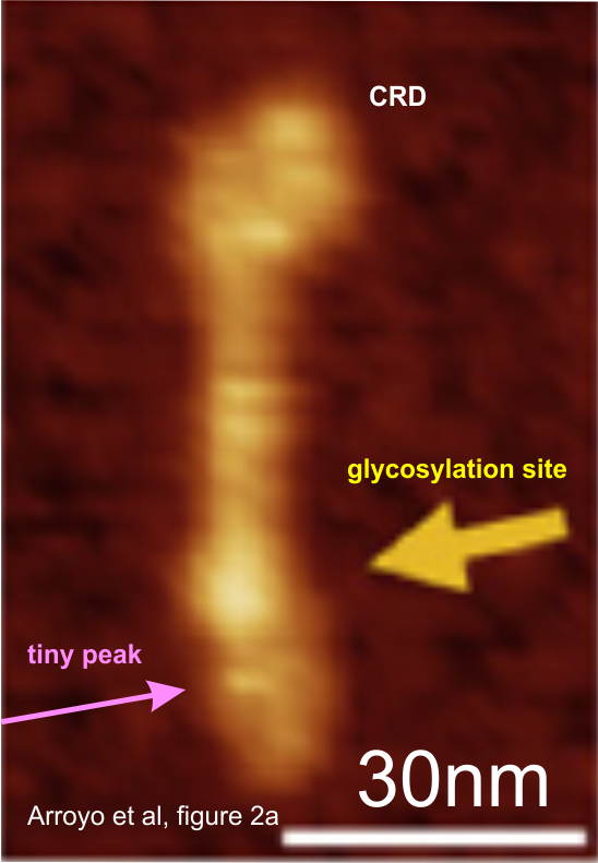
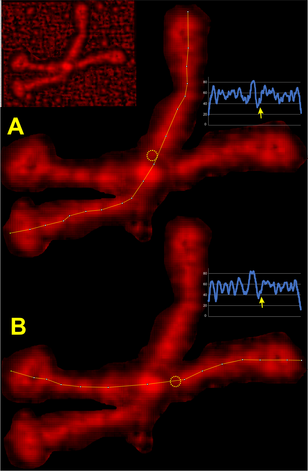
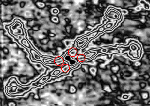
The dilemma is to figure out which data processing (as it is called in gwyddion) and called image processing by everyone else) tools can give me an accurate count of the peaks along the dodecamer arms.  It is clearly reported by many SP-D researchers that the largest (height and width) peak is the N termini juncture in the center of a multimer, and the next largest peak (width height) are the 4 CRD at the end of each trimer.

Plots confirm what my eye’s see, but I am compelled to figure out how to add statistics to the observations. Using ImageJ (FIJI), CorelDRAW (which hands down is my favorite), Gwyddion, Photoshop, and now Matlab (which is way beyond comfortable for me) I have verified that many many ways of processing the images does not in any way change what I have seen.  Yes, applying a mask or dialing down the brightness, upping the contrast,  or applying any number variations to the RGB histograms can change the number, but most images from the beginning show a number of peaks and one can watch them disappear or increase in prominence…. at will.  So when is image processing beneficial– what amount of removing background adjust for scan lines, correcting the data for scars and artifact is sufficient.

In retrospect, this project could have been just as valid if i had opened hundreds of images in photoshop and upped and lowered the contrast and brightness to a level i “liked” and hand counted the peaks…  really. Then comes the sad answer, why am i doing this, to please some editor of some journal.

It would be ideal (nothing is ideal):

1- to have programs provide (and maybe they do, I just have not found it) documentation on which algorithms they use when inter-converting RGB or CMYK or grayscale or changing HSL or histograms.

I bet this image (arroyo et al, which appears in the body of the paper and also in the supplement) has been studied, measured, and processed in more programs than any other dodecamer in history. Every nanometer of it has been examined and every striation artifact in the background looked at, (original arrow in figure covered too), peaks heights, widths, square nanometers, relation to other peaks in terms of height and underlying slope, numbers of peaks between the N termini and separate CRDs, declination of the peaks (2D) in each arm, diameter of the whole dodecamer, length of each hexameric arm as measured in segmented lines, images rotated and remeasured to balance scan out bias and background..in fact worked over ad nauseum.

It has been used to test arm straightening techniques, measure angles (acute and obtuse) of the four arms, to predict where the coiled coil of the neck tucks under the CRD, to find the tiny peak between the N termini junction and the first large peak on each side (allegedly a glycosylation site). Programs used are dedicated image processing programs such as gwyddion and imageJ, and non science-dedicated imaging programs, but nonetheless extremely useful CorelDRAW and photoshop.

All just to figure out clues that will help someone else see exactly what shape the collagen-like-domains can be modeled to.

After having looked seriously at many many SP-D images (AFM, rotary shadowed, negative stained) and the shape in LUT plots at the end of each dodecamer so consistently have a teardrop shape that it is hard not to make the association between that and the partial molecular modeling of SP-D.

It is really hard not to see the correlation.  Top four images are the original from a figure by arroyo et al (top left), RGB saved from gwyddion, bottom left, 1D fft, bottom right 1D horizontal fft (i dont know much about fft (yet), but it is clear that the teardrop shape does not go away with many kinds of image processing.  I may represent the folded distance in nm of those two domain (neck and CRD).  Another thing that is common is the narrowing of the neck coiled coil at the change to the collagen-like-domain. One can contemplate whether the collagen like domain is more tightly wound than the neck as seen in countless images of DP-D and whether the dimensions from the edge of the CRD to the neck can be measured using plots.

Panel below is an enlargement of identical segments from each of the four pictures above, one has overlay of SP-D neck and CRD, as imaged in RCSB.

Bottom panels are portions of middle panel, just enlarged and with molecular model overlying (in this case) the vertical fft transformed image.

It seems to me that this small peak in the LUT plots of many many SP-D dodecamers might be real. Images below are all derived from original AFM ( screen print from Arroyo et al) which has been measured for size as a diameter using their bar marker) and as spline curves, one for each hexamer – CRD to CRD, and has been also photoshopped to increase contrast. That image was imported into gwyddion where the it was processed with “presentation>local contrast” to produce a highly contrast enhanced image. This image was plotted (again with a spline curve) in ImageJ and the peaks are marked with dotted lines in arrows. The precise plot line is shown as a screen print and the actual plot exported to excel, imported as a metafile into corelDRAW, sized to the original spline curve in ImageJ is a blue line overlying a cropped, background removed, image.

Clearly these tiny peaks are not really visible in the original image and image data processing was required to make them visible.

I have posted other images of this small peak here and here.  It shows up in images and along the plots a sufficient number of times to suggest that it is not distortion, drag, bounce, artifact, but it is not always present, likely due to the forces during preparation. rotation. I dont know how the probability for opportune orientation and the expected number of times it is visible might be calculated.

I went back to the original Arroyo et al publication to see if there was mention of this tiny peak, and i did not find any. They alleged glycosylation site is so prominent that it is almost always visible and the width is in the 10-20 nm range, this tiny peak is not so easy to spot. However their image of a trimer clearly show, in the correct position, a small peak but it also shows along the trimer  closer to the CRD several blips in parallel, like artifact.

16:6:1 (settings for presentation>local contrast> kernel size (16) pixel depth (6) weight (1) in gwyddion) and a second set of settings  16:4:1 might be the bests processing for registering peak height that i have found.  it doesn’t just seem to be a brightness contrast change as available in photoshop. I dont know the algorithm but bet that an online gwyddion chat group could provide them.

What i observe from the LUT plots in imageJ after being processed for data processing>presentation>local contrast? 16:6:1  that the plots have each of the suspected, regular, peaks at a value that can easily be counted.  So in this particular image (also from Arroyo et al) the “best fit” plot for what my eye tells me is the left side of of this particular dodecamer, in particular the lower left arm. The real work comes in figuring out “what are the odds that this molecule will fall into perfect alignment to predict peaks along the collagen-like-domain” Each LUT plot beside the tracing in imageJ. Please not the little yellow circles = aka “new peak between the Nterminus and the alleged glycosylation site”.

This image (originally from Arroyo et al supplemental figure 4B) has been processed to the limits using four programs: Photoshop, CorelDRAW, ImageJ, and Gwyddion.  It has been converted from screen shot to jpg to tiff to png with who knows what algorithms, and I have adjusted the contrast in photoshop and exported to tif and opened as RGB in Gwyddion, and >basic operations>volumized in gwyddion (bottom image) to count peaks along each of the trimers, and compared with an additional contrast enhancement in photoshop.  And in this particular unique dodecamer (where the N termini of the hexamers are joined side by side instead of the more often found end to end through a central point) there is this cute little tiny peak before the first large peak (which has commonly been called the glycosylation site.  (see in three (marked, but probably all) of the four trimers the red circle identifying this small brighness (luminance) peak between the N termini and the major 1st peak along the arms) – top image) and all four trimers show this tiny peak in the volumized image (red circles in the bottom image).

In addition, it is clear from the contrast enhanced (by photoshop manipulation) that there is a declination present in the peaks nearest the CRD.