I think there is something very basic about the way molecule fit together that is beyond simple, just convenient. Think about assembling 2 of something… there is almost always a long and short part, or four of something, then we have a hole maybe, especially if the object is slightly irregular in shape. BUT THREE, the magic number, slight turns and little twists and the sum of the three is much more than the numerical sum.
Daily Archives: January 10, 2019
Slightly changed method for obtaining LUT tables for SP-D
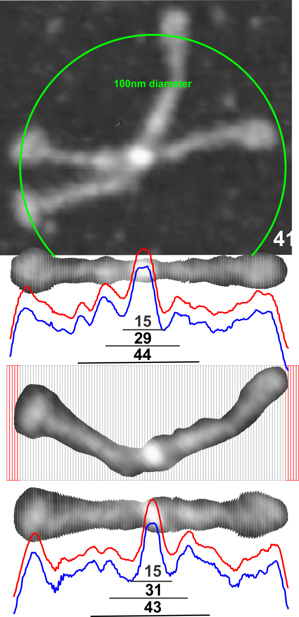 This is a simpler method for determining where the peaks and valleys are for the bright spots along the arms of the SP-D dodecamers (actually measuring both monomer arms end to end at the same time with the same N terminal juncture bright spots)
The cuts have been aligned with the 100nm marker for this particular AFM image and actually cut the image in 1nm slices. This is done using just before beginning of the greying of the two CRDs as the outer limits of the 100nm range (keeping in mind that the actual measurements made by many researchers is just ove 100nm for the width end to end of the dodecamer. They are just slightly over 100nm but I thought using 100nm as a standard (at the margin of the CRD would be an easy measurement to use as an enlargement constant (or control for the varied micron markers that researchers post that are clearly off the mark). It is my feeling that there are variations in prep of the SP-D dodecamers, but that basically the structures can be normalized to just over 100nm.
So when the sectioned areas of SP-D arms are cut into 100 slices, then the center of each of those slices centered horizontally will the other slices…. the light and dark areas are ligned up (as shown in previous posts) but NOW each slice represents 1nm. This makes it incredibly easy to measure the distances between peaks and valleys of the correspond look-up-tables, align them in the same dimension width-wise, and determine bright spots as well as how many nm they are separated from the CRD or N terminals. It just requires an aligning of the two plots under the image, and using the select tool to select however many 1nm segments occur (automatically counted as “objects”) within the selected area.