Monthly Archives: February 2019

Silk nanofiber – LUT plot worked well

Looking for AFM images of CL-43 and SP-D and A and MLB and conglutinin i ran across this portion of a silk nanofiber and tested the centering and plotting of LUT tables using CorelDRAW and ImageJ.  Looks like a nice plot.. took less than 5 minutes but supports the methodology. Red line is the LUT plot, over the original slightly curved fiber, top is cut into 300 slices and centered, then exported as a TIF and the luminence profile plotted in excel and superimposed.

Plots for peaks in arms of SP-D dodecamers

Plots for the second dodecamer arm in an image publishes by Leth-Larsen et al,J Immunol 2005; which seems to provide similar counts of LUT peaks within the collagen-like domain of SP-D. I analyzed the first of two SP-D dodecamers in the AFM published images. One half arm with 1, then 2, 3 and 4… so all over the map.  Plots were taken with 500×25, 500×17 and 500×1 pixel rectangles and superimposed upon each other. Two arms analyzed separately as on 500px length=100nm.

Counts by and (with out the LUT) were similar to peaks.


So many variables: shadowing, rotary shadowing, AFM cantilever types positions, preps

I dont know how anyone makes progress. Some materials and methods dont really describe in much detail what processes are used to produce such images. Whats more problematic is that there is no even consensus amoung journals about how best to show the images and image properties, or even something as simple as a standard for micron markers.

There are standards out there. I know I used to have a grid to establish the magnification (which then had to be calculated back from what pole pieces and objectives I used, but I still tried to do that). Even when markers are present they are obviously off even according to the accompanying text.  Whats more, there was no standard way to put the magnification down for light micrographs… we used to say, “original magnification” 100x, which could mean absolutely nothing depending upon print mag, optivar, objectives camera magnification and whatever.

1. Electron Microscopy Sciences.
2. Electron Microscopy Sciences
3. Electron Microscopy Sciences (for AFM)

Measuring peaks along arms of SP-D dodecamers

Measuring LUT table values (lluminance peaks) along the arms of SP-D dodecamer images taken with AFM is almost a no-brainer. Though peaks are not always evident by eye, they show up as a classical peaks in the LUT plots (A peak is defined as one point higher than two adjacent values, haha,  I think i will use more than one point higher, but that is the definition). The AFM images are so good for showing height of a molecule that way that rotary shadowed images are certainly NOT.  I have used mostly AFM images to try to convince myself that there are three peaks of graded luminance values along the collagen-like portion of the molecule.  So this uses about 18 separate images found in the literature. 18 is not big number, I would love to have 100 more. But the rotary shadowed images dont even come close to showing that particular type of detail. But today I wondered how to make a “background” to be subtracted from each of the larger round bumps along the rotary shadowed…. I am thinking perhaps it can be done with “diameter”… that is establishing a mean diameter for the shadowed particles in the background and counting anything more than X% above that, a possible peak. The background diameter (derived fresh from each image) line could be drawn along the straight OR curved length of the SP-D arms as a line,(right down the center) and any deviation from that background diameter could be considered an “increase”, the amount of increase could be calculated by difference in the areas. This is a TEM from someone’s paper, i am too tired to find out whose… LOL, but it is possile to see differences in background lump size…. most evident obviously on the CRD, less evident at the N terminal (which is so different from the AFM images, but the diameter of the arm stretch could be measured.

So I just happened on this particular example which I used (red line) and the background luminance height (blue line) and there are really four peaks above the background (nice, but waiting to be repeated in the dozen other arms I should measure.  This is just ONE HALF of one arm. N terminal is marked on the left CRD is marked on the right (and clearly the largest area and highest luminance.  This is different than the N terminal in the AFM, where the latter is the highest in luminance and also at least the same diameter as the CRD. It is time to look up the mechanics of shadowing molecules for TEM.

Collagen like domain in SP-D

I don’t know why the collgaen-like domain of SP-D keeps being labeled “disordered”  It is highly ordered as seen in shadowed and AFM images. This confuses me.

See red line area midway down under the section “disorder”. Aside from the fact that the collagen like domain is “ordered”, the idea that “disorder” exists in any of these highly specific and well adapted, and very old proteins is just a little naive. Kind of like looking back in retrospect at the guy who first coined the term “junk DNA”  ha ha.  Not gonna be so, ha ha, and reflects lack of knowledge rather than any biological disorder.

Reminds me of a lecture by the Late Dr. Ernest Foulkes, way back in the 1980s when he was working on metals and kidney function. I remember so clearly his statement, when the kidney was overwhelmed by whatever metal treatment he had given, said… “looks like bad design”  EYE ROLL.  ha ha… like he could have come up with something better than what nature devised over millions and millions of years.  Also, not gonna happen.


Does von Willbrand protein diagram fit the AFM images?

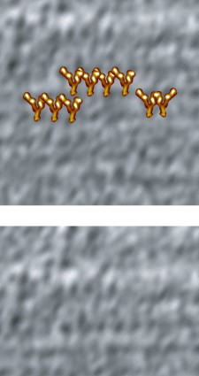
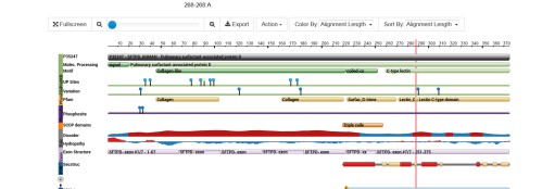
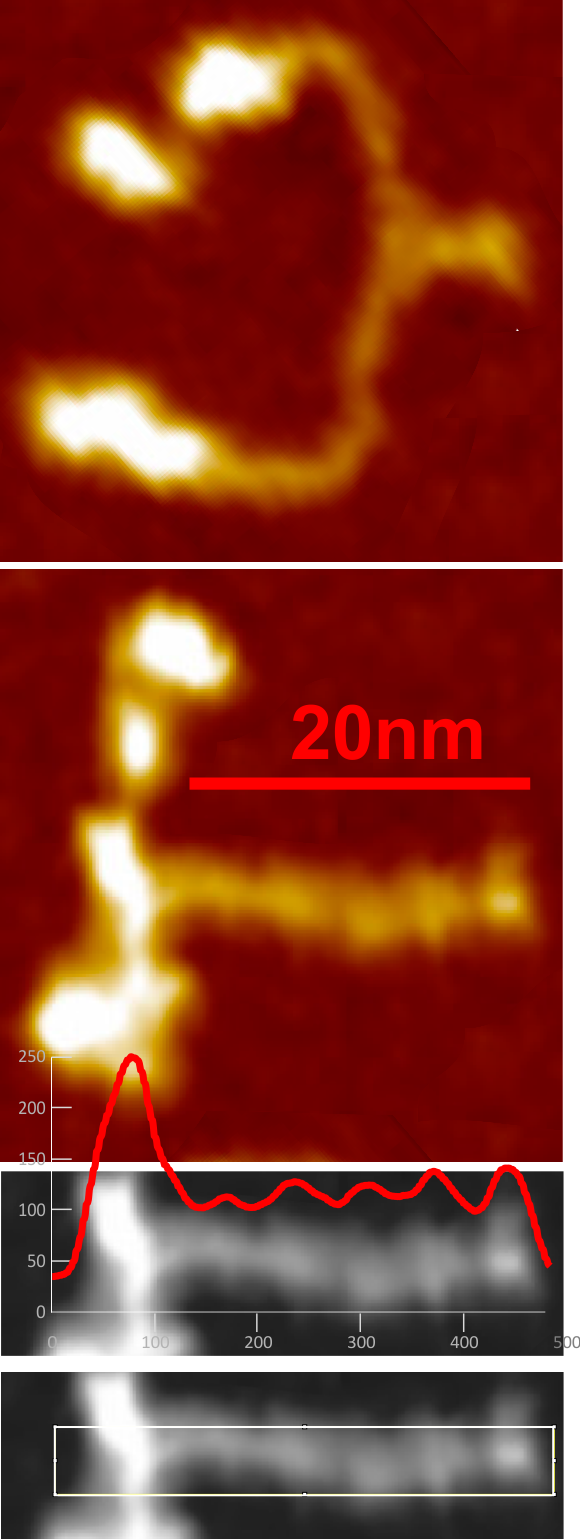
Lof et al, (Plos 1 Jan 2019) shows two monomers as a diagram of two molecules of von willebrand protein at a point where the winding portion is drawn apart.  The actual AFM images look to me like the molecule winds up from the C term, and it makes sense in terms of ease of unraveling the molecule into the extended state at the beginning of clot formation.

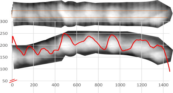
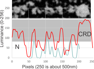
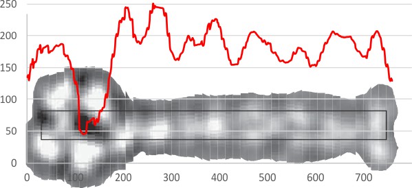
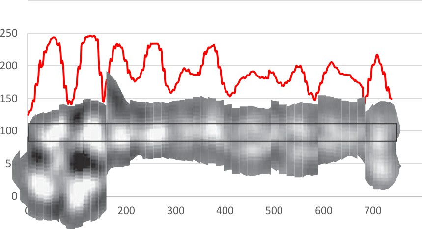
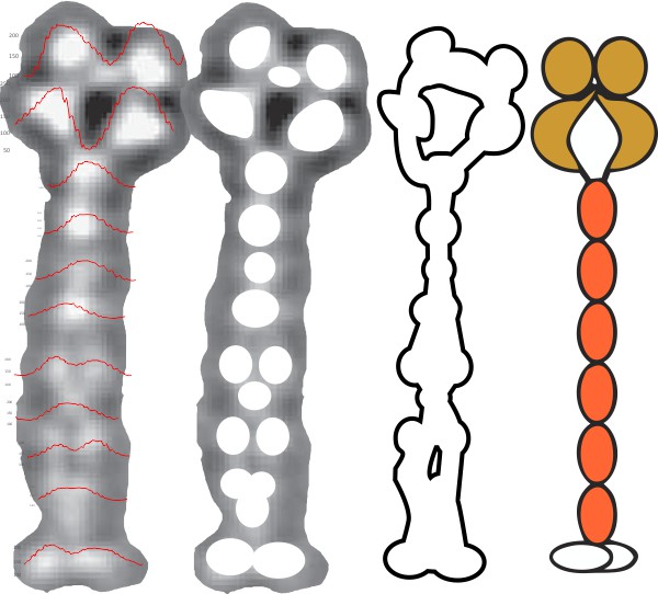
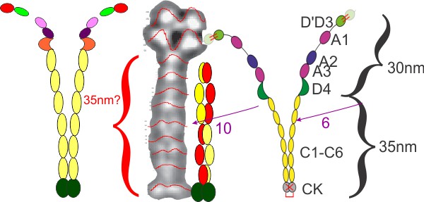
Issues remain between diagram and AFM image: the diagram (even though the domains are named as C1 – C6) and puts six vertical ovals in the diagram, I also don’t see that number of densities (which plot on the LUT tables, in fact there are more, in addition to the clear appearance of two peaks in the LUT when lines for analysis are drawn horizontally on a vertically oriented image. Also, the  top of the wound monomer in the AFM image is nothing like the diagram they show. I acknowledge that I might be missing something but the images look very different than the diagram (see their diagram on the right hand side) my analyses of LUT peaks in their image and measurements of theirs are certainly not the same proportions as the AFM image.

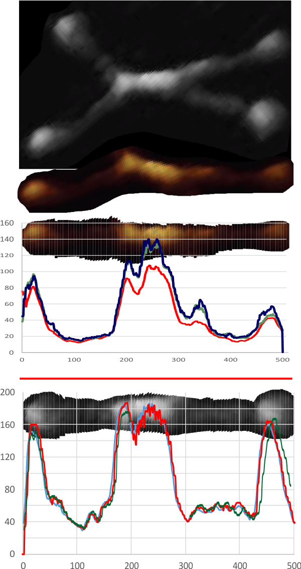
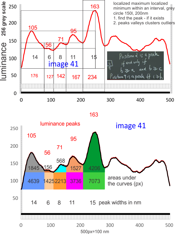
Here is a comparison image, my graphs on the right and my LUT on the image from their paper (they published four images which had the same one spot, two spots,  one spot, two spots — patterning in the “stem”.

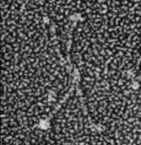
Other authors (Berriman et al, 2009 PNAS) uses electron tomography to make a great “…..lattice drawn on half the pattern (their Fig. 4B) which shows that the VWF tubules are helices with a repeat of 360 Å in which 13 subunits make three turns (about 4.3 subunits per turn).

here is a great image of the granule (Wiebel-Palade body) in a publication by Berriman et al (PNAS) in which a very orderly form of tubules stores this protein.  Great micrograph…. would love to do some organizing of molecules on this granule pix.  ha ha.

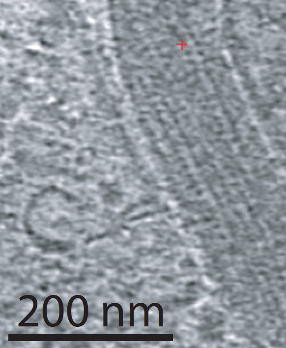
Dimensions of the shadowed molecule and the Weibel Palade body, don’t work out easily. but here is an approximate size highly wound up VWF protein over such a granule …within a granule, which can be a highly organized tubular structure….

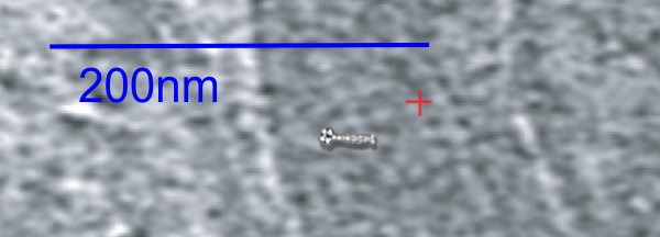
This is just a wild hair…. looking at the periodicity in the electron micrograph and possible positions for a regular alignment of VWF in these Weibel Palade bodies…. Nothing scientificaly produced here just an image that looks right over an image that looks right…. ha ha, magnifications are not that far off… I think there would be vertical lines (as one sees in the Langerhans cell-birbec granules) were the VWF wound up at the C termimals (CK) to whatever binds them at D4. What is interesting is the alternating position of the densities along the margins of the tubules creating the illusion of the Y shape in the granule.

More thoughts on von Willebrand protein structure

When i saw this article by Zhou, et al, in EMBO 2011 I was curious about the shape of this really fascinating molecule, von Willebrand factor.

My first thought was to cut them up, straighten them (though many of the tightly bound short (non extended) though the molecules do look pretty straight and rigid (per their article) I did it anyway seeing if i could bring the four bright spots at the N terminal part of the molecule (i dont know that much about this protein, and the paper gives lots of details that I did not search out so i have to assume they are right) into a horizontal alighment to make a zig-zag LUT table for luminance.  After looking at their images for a while I noticed that there was a huge discrepancy in the way the molecules were plotting out and their diagram. These are my observations.

  1.  I count 17 and maybe 18 bright spots along the molecule (see figure below), they only count 12 (for reasons unknown)
  2. I find two places where there are definitely two peaks (two bright spots, they only find one) (for reasons unknown)
  3. With LUT plots superimposed over the areas they measured  I don’t see any reason to ignore the areas where two distinct peaks are present.

These are really nice images in their article, but i think more could be found in them. My horizontal LUT plots are top and middle images and the vertical LUT plots are on the bottom figure, plus what i think are the bright spots (correlated with the plots to the left) and a construct just from those bright spots at the center right, and their diagram on the far right.  You can decide.

More fascinating molecules to test out this morphometric method: von Willebrand factor

von Willebrand factor, according to the publication from which I examined the AFM images of this dimer linked HERE, is a “force-sensing” dimer in blood that under conditions of increasing hydrodynamic factors can be activated to bind platelets and collagen.  AFM images provided in the manuscript look like what is a W shaped dimer becomes a T shaped dimer with the winding up of the inner arms of the W, tightly, and and unwinding as well that adds a whopping 80nm to the length of the arms and they say that this protein can get up to 15 microns long in plasma as linear multimers they call concatemers (think twisted yarn, pulling apart lengthening, then when tension is released winding back up to a single dangling fatter arm (haha or anyone who knows the twisting of the old phone cords in to winds that unwind and wind back up..this looks similar to me — and it makes sense that a force can unwind it)  von Willegrand factor is a large glycoprotein found in plasma.

Like SP-D, which is the reason that I am looking up these AFM papers, mainly trying to apply a morphometric method to various molecules) von Willebrand factor is linked by its N terminal (what a surprise, ha ha).

One interesting thing that was mentioned was a “step growth” in multimerization, adding two molecules at a time (kind of like adding one dodecamer at a time to fuzzyballs of SP-D)

Here is the image from Muller et al, which I have cropped to show the LUT tables for the tight end ( the C terminal joining of two monomers), the base of the “Y”. In the plot luminance is the ordinate, length is the abscissa a should be derived from the red bar marker, whole molecule X factor is pixels. (Super easy to do and really nice, showing these winds, almost as if the think were really coiled up on itself like twine or for those of you who sew just thread, or for those of you who embroider or do needlepoint, just like floss). Nothing surprising there, but that is one-tight end, the tension in that molecule is almost palpable. Tomorrow the open molecule will bet measured and LUT worked up, looks like two turns already.

Perhaps these 5 approaches are the best measures for AFM images of SP-D

In the diagram below I have highlighted possible measures of SP-D images (AFM) which might shed some light on how many peaks are in the LUT tables, most particularly in the collagen like domain. It is obvious that the CRD and the N terminal junction of two trimers that make up one set of arms of the dodecamer are easily seen and not that variable (with the exception of the lumpy character of the CRD which sometimes shows a smaller peak in the luminance on the LUT tables.

  1. pixels (area) beneath the curves (separated from each other at the side of the value for the lowest valley (which almost always ends up on the outside (lateral) edges of each peak
  2. distance in nm of each peak (100 nanometers on the x axis)
  3. peak height from 0 on the luminance (1-256 on the y axis)
  4. peak height from the lowest valley on each individual portion of the LUT tables
  5. hand counting peaks (in this case 9 total with two of the peaks showing a tiny sub peak) but 3 on each of the collagen like domains and one in the center (N terminal juncture between two SP-D trimers) and a CRD on each outside end.

The typical number of peaks in any dimer-arm (two trimers end to end at N terminals) is measured at 100 nm and equals 9 i believe.