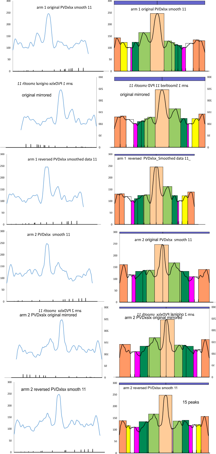
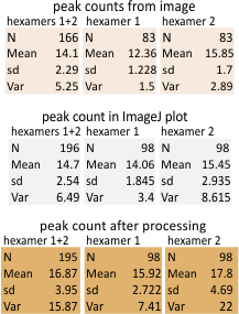
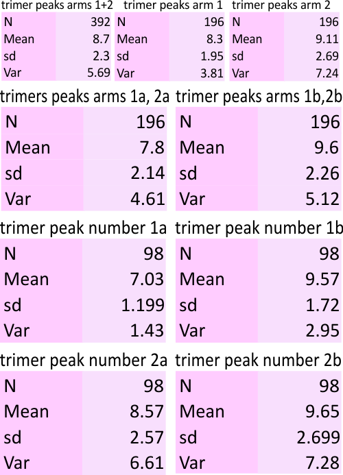
11 peaks (brightness/grayscale) traced along a center, 1px line in a surfactant protein D hexamer is the absolute minimum that can be easily described. Furthermore, and routinely, as many as 15 peaks can be found. More are seen with different algorithms, but may not be consistent. Much depends upon how the molecule falls, the over or undersaturation of the contrast (in the original and in the image processing), and the quality of the image (obviously). Also, critical to finding peaks is the care with which the segmented line is drawn (the greater attention to this is what produces two peaks (sometimes 3) in the center of the N termini junction, and in the area just before the N termini junction (i.e. the area between the glycosylation(s) site and the N termini – which i have referred to in several posts as the “tiny peak”).

Thanks to Arroyo et. al (2018). (about 90 images of SP-D) and Thomas 0’Haver and Aaron Miller and Daniel Miller (numerous signal processing programs and algorithms) for their contributions of numerous signal processing programs and algorithms.

11 peaks is just the simplest count from poorer resolution AFM images, using just the most basic image and signal processing tools which are freely available to anyone. But careful analysis and fine tuning images with gaussian, median, mean, sharpening, and range limiting filters, as well as optimizing options such as smoothing, lag, threshold, width, influence, etc  in signal processing shows the peak number to be close to 15+ per hexamer.

One of the surprises of signal processing plots from ImageJ is an apparent disadvantage in peak detection in being a molecule with large differences in peak brightness, coupled with prominent bilateral symmetry.
In the sense of perception of mirror symmetry has significant functions human perception. It has been shown that symmetry is detected within randomly placed elements, and it would be an easy leap to see this visual function as evolutionarily advantageous. Whats more, subjectively speaking, symmetry is apparently pleasing (using self as a sample) as I do this in my own artwork, and see it in architecture and other artwork as well. Not only symmetry but repetition (particularly iterations with rotation) and nature does this supremely well, and it has been studied mathmatically. Instances are too numerous to list and readily available to search online.

An interesting attribute of human sensitivity to mirror symmetry is “tolerance” to error, meaning that variations dont matter a whole lot. This may relate to the extreme abuncance of what biology does with duplicate molecules in arranging them into dimers, trimers, etc on ad nauseum. I am thinking that my interest in surfactant protein D, which has so much “symmetry” (not unlike other patterned, replicated, duplicated, inverted, rotated, molecules found everywhere), and just enough noise may be a visual symmetry puzzle, at best.

What is exciting is that SP-D runs the gamut of everything from monomer to multimer (multimer here being that unique molecule named the “fuzzy ball” by some surfactant protein D researchers, which at any point can have 100 or more monomers). In time, such a multimer will likely show numerous mirror, rotate, iterations which can be seen at quick glance before any image or signal processing.   Just for fun I re-uploaded a graphic mandala that I made a couple years ago, which is a “fake” look at fuzzy ball symmetry (12 trimers, 36 monomers. Alleged glycosylation peaks are a dark blue ring arou the center, CRD are the bumps at the ends of the molecules. Actual SP-D image, masked and colored in CorelDRAW. Pink background, black, white and blue abstract borders are “fills” and not relevant to SP-D structure. Artistically speaking i should go back and edit the background and border for more pleasing texture tile settings and colors. (LOL) and rearrange in the trimers.  Even in this artsie craftsie image the peaks along the arms can be seen. I am not ready yet to relegate the entire interpretation of the shape of SP-D to the best image and signal processing programs. Human input is obviously required still.

Apologetics: I am tired of trying to find a way to calculate peaks and valleys of this protein in a way that might be considered “biasless”.  Great quote I confiscated from a valuable signal processing website gave me inspiration to make a re-do of it.

“image and signal processing do not substitute for judgment, any more than a pencil substitutes for literacy” modified from Robert McNamara.

That said, I have made (with image processing in gwyddion and photoshop) a really nice image of an SP-D dodecamer and so clearly there are about 5 bumps in each of the CRD domains, a funnel shaped bright spot in the neck domains, smaller (and also thinner) peaks along the adjacent collagen like domain, and variable lumps and sizes for the area of the collagen like domain which is believed to be glycosylated.  THe lumps and bumps in this peak area appear to me to be due to the possible partial glycosylation (one, two or three) of each of the trimers.  Then there is the tiny peak which very often shows up right in the valley between the site of glycosylation and the typically very tall N terminal junctions of the four trimers. The latter (shown in this image) has a little depression which is commonly seen in the N peaks dividing that central area into two separate peaks, and even in some cases with a smaller elevation between the two.  All in all, I didn’t need signal processing of the peak plots to see this, and only used the basic filter functions in CorelDRAW and Photoshop to make them stand out.  Lots of effort went into the “image and signal processing” which has taken about two years, and was really not that informative to ME, but was just required to satisfy the predicted onslaught of “bias” comments.

Here is the image described above (41_aka_45, mentioned and shown many times in previous posts on this blog). White arrows and circles point to details mentioned above in obvious places, but all can be found in countless other images of the trimers.

It seems likely that one of the reasons that the tiny peaks on either side of the N termini junction of a surfactant protein D dodecamer when employing signal processing is that with the enormity of the N termini peak the requirements for an adjacent peak are too great.  I think in some kinds of image processing this might also be a factor, maybe those which “sharpen” in particular, but it surely must happen in some comperable fashion.  I really noticed it more in the signal processing algorithms than image processing.

Also missing is the splitting of the N termini junction peak into two (sometimes with a very small peak in the center) using the signal processing algorhythms. Maybe for similar reasons.

It is a little distressing to watch the signal processing algorithms continually pass over a peak that I have seen many times in many molecules, and then say there are 4 peaks in a short span ot distance where there are literally “no peaks to be seen”.

In thinking about signal processing programs for analyzing plots of grayscale peaks and valleys from traces (made in ImageJ) of SP-D molecules (AFM, an image published by Arroyo et al) I was sort of surprised to see that sometimes what I would call “nonsense” peaks and valleys showed up, and others i thought should have been counted were left out.  This only surprised me because I dont understand the algorithms that are used to predict peaks…. i understand that. But I am not willing to let go of what my eyes see as a peak, to some that doesn’t understand the greater symmetry in biology, and in particular, in the dodecameric structure of SP-D.  I took one image, and plotted both hexamers in both directions.

Previously when plotting in Gwyddion it was evident that the plots were not reproducible when the image was rotated 45 degrees, so these plots were made in ImageJ, and those replicates seem to look pretty much the same.  (see figure below) the original tracing in imageJ  (1px line) left to right through both hexamers.  The reverse plot went from right to left (but the arms were given the same names (1, and 2).

This first set of images is processed (5px gaussian blur), plotted in ImageJ, exported to excel. Peaks and valleys were selected by hand. Top set (original plot), second line, those plots mirrorred, third line, plots in reverse direction. Colors: peach (N term junction); purple, tiny peak so far undescribed; light green peak is likely the glycosylation area; dark green, pink and white peaks not yet defined; yellow and orange, neck and CRD in varying orientations. The hexamer is allegedly bilaterally symmetrical so peak heights and widths and numbers should be consistent. BUT in at least two instances they wont be, that is at the neck and CRD since there is a host of different ways that those three CRD can fall and be arranged during processing; and the glycosylation peak area may reflect different heights widths and lumpiness depending how many sites are glycosylated.  In the arm 1 below, one glycosylation peak is considerably lower than the other and this likely is meaningful.

The second set of images (not shown yet) will be made using the same arrangement, but an excel template PeakValleyDetectionxlsx (Thomas O’Haver) arranged in the same way.-, with same color arrangements. While I would have liked to see the valley markers at the beginning and end of the valley-plot produced (black line at bottom shows where valleys are calculated), cropping the valley series at the bottom of the plots at the same point as the length of the plot of the peak series helps make the last peak an appropriate width. The forward and reverse plots (compare the reverse plots at the bottom with the middle set (mirrored plots), show quite similar data. In fact, where I draw the segmented line accounts for the greatest differences in peaks size and number as that line grabs the grayscale values.  Such differences in peaks/valleys occur in the plots of the N terminal junctions  (center peak, peach color).

Finding peak height and width from image plots (ImageJ) and signal processed plots (Octave and Excel templates)  can be done, but by and large, trying to figure out any details for where the markers for the widths of the peaks  in the signal processed plots is no better than doing it by hand, EXCEPT for one excel program which is free to anyone developed by Thomas O’haver, and is called PeakValleyDetection.  This program allows a new series to be plotted which shows the valley marks on the plot.  For me, this is the best program so far for determining where the valleys are “without my personal input”.  Looking for valleys and peaks in all other measurements seems to be a mattern of “selection” by the user.

Here is an example. 1) original image and plot using ImageJ, 2) plot from image J smooth using PeakValleyDetectionTemplate-xlsx, 3) comparison plots from my choice of valleys and peaks within the ImageJ plot and the valley choices made automatically by a smooth factor of 11, in the PeakValleyDetectionTemplate-xlsx. They are close.  I made some different choices, and the algorithm made some as well. One issue with the xlsx template is that it tends to leave off (or not count) the last peak. I dont think this is a good thing, but I bet that the problem is that it uses a “backlooking” perspective and does not account for the fact that in biology there is so much repetition (mirror, duplication, inversion, tandem, bilateral, etc etc ad nauseum) that iterations of a pattern are not taken into account like they should be.  This is one of the reasons that the plots were analyzed as trimers separately.

OK, a new issue just came to mind – and that is a) the segmented line used for plots always went from left to right, and therefore in the algorithms, there may be some bias, whereas with the human eye, probably not.  So that begs the question, if i plot all trimers outward from the complete N termini peak, will this change the results in those plots which plotted in the mirror of each other.

This is the beginning of width and height counts for the summation of numerous measures of many image and signal processed plots for a single dodecamer. (see previous posts) and image of the actual dodecamer at the end of this post – a guide to labels and names used in the summaries).

Starting with the width of the N terminal peak which is a junction of four N terminal domains from each of four trimers, thus 12 parts. Results in nm (calculated from the bar marker in the original image).

No variation here in the width of the N term peak regardless of how one measures it. It appears that going from one side to the other within the context of each arm shows an even and regular arrangement of the three trimeric N’s.  When measured individually, the same results appears. Some of my original counts did NOT include a tiny peak on either side of the N term juncture and this accounts for the change from @20 nm width to the current value of @15 nm.  The appearance of that tiny peak resulted from the use of signal and image processing tools.

Just to reiterate: these are all values from analysis of a SINGLE SP-D image (noted many times before in this blog). Various methods of enhancing the image for detecting peaks (whether by filters and masks in photoshop, corelDRAW, or corelDRAW photopaint, or Gimp or gwyddion, and several more raster adjusting programs, as well as a few signal processing programs (PeakValleyDetection xlsx, PeakDetection xlsx, Octave (ipeak.m, findpeaks.m, allpeaks.m), there is concensus. IT IS CONCENSUS BY CHOICE. It has to be recognized that the CHOICE, whether of filters and masks in image processing, or functions in signal processing, is mine (YOURS). Peak counts can be manipulated to go from 1 to 40 in both image and signal processing. It requires sensible input from the user.  That said – 15 peaks per hexamer looks pretty solid.

Here are the N, mean, sd, var for trimer peak counts – which numbers include the processing that has been done so far, so this will change with other variations on the signal processing data. Please note that the complete N terminus peak is included in the counts of every trimer (this means that from the distal edge of the center bright peak to the CRD is what is measured, so counts include the whole N term of the dodecamer as a ONE peak) in each trimer.

I happened upon this website, saying alpha fold is helping with protein structure, which it probably is, but it hasn’t helped with the structure of SP-D yet —  as the areas of low significance (orange and red) are completely out of line with any microscopic evidence (see AFM from Arroyo et al) which shows nice correlation with the blue areas (high probability of being correct) vs the rest of the model which has absolutely no correlation with the shape of the rest of an SP-D trimer.  Images as presented in this model (proposed models left hand part of the figure below) are the reason I continue to try to establish an accurate count of the number of peaks, their height, and width, using various imaging and signal processing programs to help define the shape along the more or less “straight” collagen-like and N term domains of an SP-D trimer.

Carbohydrate recognition domain and neck domains (BLUE) are spot on, collagen-like domain and N termini junction (orange and yellow)… really really no good.