The choice of what algorithms to choose for analyzing 100+ surfactant protein D images (AFM) will amount to selected image and signal processing functions. 6 – 10 plots will be made for each hexamer of a single dodecamer.  The concensus plot to which to compare all these plots will come from a concensus of peak number, and peak widths and peak heights from these data.  A composite ridge plot created from a single molecule (41_aka_45) (below) indicates that very predictable patterns of peaks and valleys do occur.  That said, it is pretty certain that there in an ideal tracing of a trimer there are 7 peaks, and something around 15 in a hexamer (which depends upon whether there are portions of two CRD in the tracing and two peaks found in N (which does happen).

1. maybe two peaks at N
2. two tiny peaks on either side of N
3. The glycosylation peak man NOT be just one peak but a set of rolling peaks – as the number of carbohydrates goes from 1, 2, to 3.
4. a consistently appearing peak peak similar in size to the glycosylation peak located on the lateral sides of the glycosylation peaks, and
two additional,smaller, as yet unnamed peaks, lateral to that peak and before the neck domain.
5. Occasional appearance of a peak related to the neck domain, dependent upon which direction the globular carbohydrate recoginition domains lie during processing.
6. One or two large peaks of similar width and height occur on either end of the hexamer (depending upon the positions the carbohydrate recognition domains fall into as they settle during processing.

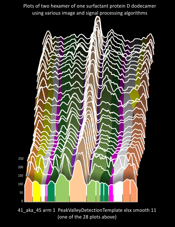
Image processing:
ImageJ for tracing all plots
one image unprocessed
Photoshop 6 for sizing, dpi, contrast and gaussian blur (5px or 10px filters)
Gwyddion for gaussian blur (5px or 10px) and limit range (@100-255)
CorelDRAW x5 for graphics and normalizing plots, dividing plots into trimers,

Signal processing:
one image unprocessed (other images image processed as above)
PeakValleyDetectionTemplate-xlsx-smooth 11
Lag 5 Threshold 1 Influence 0.05 (?Stackoverflow I dont know whom to credit)
Octave, Ipeak M80
Scipy (Prominence 0.2-Distance 30-Width 5-Threshold 0-Height 0)

Data collection:
Excel and Calculator.net

Peaks will be traced as hexamers using a 1 px segmented line, always left to right, and always with an ID of which arm ( hexamers (arm 1 and arm 2), and trimers (arm 1a (always left, and 1b always right, etc). No rotation of the original image will be made (to randomize the traces in terms of possible warping in depending upon the direction of the line as it follows the molecule (this was a serious issue in Gwyddion – but i have not detected it so far in ImageJ), plots exported from ImageJ will be saved, plotted in excel. Screenprints of the molecule, tracing, and plot will be saved as “white paper”.

This is really a visual document of what I have found with a single surfactant protein D molecule (image of Arroyo et al, plots made in ImageJ, some programs for image processing include the industry standards (corelDRAW, PhotoPaint, Photoshop and others) and industry standards for signal processing (Scipy, Octave, and excel Templates (Thomas O’Haver, and others).  It demonstrates to me that the known peaks in SP-D are not the only peaks that will influence a model of the structure of that “trimer” “hexamer” “dodecamer” or other “multimer”. Each trimer shows what I believe to be at least 6 peaks on either side of the N termini junction peak (the tallest peak in the center of each of the diagrams below). The plots here are of hexamers – that is, two trimers with C term on either end of the plot (ie mirrored) , and the N termini junction in the center of two trimers.

The set of plots in the ridge plot (plots stacked and staggered, background black) are those obtained from various image and signal processing plots.  Sample plots (from one of the two hexamers of this particular protein (which i call 41-aka-45), are of arm 2). I have colored the peaks that are known  (light orange in center=N term juncture; darker orange on either ends=carbohydrate recognition domains; lighter green=glycosylation peaks; Purple peak=unknown tiny peak in the valley of N term juncture; darker green=unknown peak beaide the glycosylation peak; pink peak=consistent narrow and not tall peak; yellow=neck region, often seen peak that corresponds with the differences in obscurance by the CRD peaks as they may or may not lie over the alpha coiled neck domain.

Lower image=actual plots (some from each arm of the hexamer) to demonstrate how the different colors in the ridge plot have been determined.

This was an idea I got from searching how to compare grayscale plots of AFM images of varioius molecules, but in this case, that is, the RIDGE PLOT. Image below is a ridge plot of of just a few of the grayscale (LUT plot) tracings made of a single SP-D dodecamer (image 41_aka_45). The variations in the plots arise from the two different hexamers (top plots are one hexamer, bottom half is the other hexamer), subjected to various image processing filters (in numerous programs). The second source of variation would be where in the center of each hexamer the segmented line for the plot is drawn (all drawn using ImageJ).  The differences in image processing filters cause noticeable differences in peak height, but change little in the number of peaks per plot.  The basic shape of the plot of each hexamer is very consistent, but the plots for the two hexamers has greater variation.

While I dont know yet if there is a way to compare the ridge plots using signal processing (I continue to look for that) in the mean time, this purely graphic representation (unedited) shows clear evidence of consistently appearing peaks between the N termini junction peak and the peaks associated with the CRD (no new news there). But the visual information is quite accurate.

Where plots are almost identical one understands that the variations in filters did very little to change the grayscale plots, where there is greater difference, then the image processing enhanced or reduced the heights of the peaks. More variability in the plots one of the two hexamers is evident (top tracings).

Image with plots normalized for x axis and center peak centered in this image.

I will use CorelDRAW to normalize the width of the plots, and center the N termini junction.

Here is a ridge plot, each tracing staggered slightly to the right, and transparent graded color marking KNOWN, and reported peaks.  Center=N termini junction, light orange; on each side of the N term, Glycosylation peaks=green; and at right and left ends, CarbohydrateRecognitionDomain peak(s) sometimes one sometimes two=orange.

Lots of measurements, maybe this will allow me to pick and choose which processing provides what I think is the best overall measurement of the N termini junction peak for SP-D.  This includes image processing (dozens of programs and filters and masks done separately) signal processing (several algorithms from libraries used by Octave, Scipy, some excel templates and others) and a section of citizen scientists who pointed out peak number and position.

The tiny peaks on either side of the N termini junction are elusive, and dont show up all the time. Fact is that I see them frequently but only record their widths and peaks if the signal processing programs detect them. It is likely that I pick them out when signal processing only does so occasionally As for citizen scientists (1/52 plots) does not. Therefore a comparison of that image processing vs the signal processing data will be quite different. 165/632 trimer tracings (38%) showed a tiny peak (38%).  The image processing was best at detecting those small peaks on either side of the tall N termini junction peak (detected 133 times out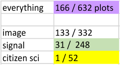 of the 332 plots made with images processed in various manners. Citizen scientists just did seem to see it.   The mean nm for that peak (actually those peaks, tiny, and at the valley on either side of the N termini junction peak) is shown to have a peak width (this is measured valley to valley) of 3.55nm.

There are variations on the grayscale peak within this molecule, which has not yet been described. I have found three variations.
1) simple smooth peak
2) two peaks
3) three peaks (this is infrequent enough to be ignored, perhaps, but I am giving you relative incidence, peak width and height anyway.
The values below are for all peaks counted in three datasets: image processing, signal processing, and citizen scientist counts.
The dataset has plots from one image removed (Inkscape, roughen inside – which produce peak numbers for the entire dodecamer which were well over two standard deviations from the other processing programs). The other change is the switching two sets of data back to normal, from the order they were traced – which was in reverse direction, meaning that the what turns out to be a significant difference in arms length overall, these trimers now the correct order.
Only 13 of the 634 (recall that four traces were removed (Inkscape, roughen inside) total plots of trimers showed a tiny peak within the N termini peak.

peak width is based on the mean nm length of a hexamer from molecule 41_aka_45. That mean, SD, median mode etc, is below (142.87 nm from CRD to CRD) as distance recorded from the plot through the center of the hexamer using ImageJ, and calculated back to the bar maker that accompanies the micrograph.  Each plot varies slightly, and the nm was recorded for each image processing filter and mask.  No hexamer length was recorded for signal processing plots, as these values are all based on the existing image data. and would constitute a repetition.

All the incidences of tiny peaks within the N term peak (not to be confused with the tiny peaks on the valleys either side of the N term peak) occurred on the right half of this particular dodecamer, likely because of some incident as the dodecamer was delivered to the mica. Whether this is something to rare has to be determined. Of the 8 occurrences (, 2 were in arm 1 trimer a, 6 were in the plots of arm 2 trimer a (2=arm 1a, 6=arm 2a).  Peak width conting so few is less than 4 nm in width. See chart below.

I mentioned in the last post that there are some structural characteristics of surfactant protein D that are accepted as reasonable (which seem pretty likely to be the case). This includes the character of the carbohydrate-recognition domain, which has a structure that is globular.  The yellow arrows (figure below the molecular model) show what kind of peaks (on an ImageJ plot) will occur in a trace through the center width of a hexamer (i.e. a line through CRD+neck end of a hexamer to the opposite end where the neck+CRD of the second trimer are).

In the grayscale plots of SP-D it has become clear that there is an assortment of peaks that occur at the CRD and neck region that are accounted for by the positions of the CRD as they dangle from the coiled neck domain, sometimes lying atop each other, or side by side, or over the neck region completely. One can anticipate that two peaks at the end of a plot of a trimer might represent one CRD domain lump and a peak of lesser height as the neck domain. Other times, there will be two peaks of similar height. In these cases when I observe the plot superimposed on the image it is clear which peak is aligned with which domain. I have given the peaks separate colors, as I have sorted them out during this project.

You can check out many previous posts where I have sorted peaks by domain (aka color), both known peaks and those identified but not named (the colors have been pretty consistently assigned during this process). Image on the right is what RCSB shows for the CRD+neck end of a trimer of SP-D, and even in this ball and stick model (colored by amino acids), the density of the transparent image shows one that a grayscale plot could show brightness peaks (and it does show them) where there are two CRD overlapping.

The image below is a dodecamer which has been image processed with a gaussian blur and a grayscale limitrange of 100-255. I have superimposed the transparent CRD+neck ball and stick models over the end of an image of a dodecamer (arroyo et al) (41 aka 45 by my number). Yellow arrows show where several peaks in one CRD region will be found.

Looking at the middle, and brightest area (the N termini junction) there is a slightly darker center in that peak which is often detected in peak counting. In addition this molecule also has varying brightnesses of the glycosylation peaks (in particular compare the lower right hand trimer with the upper right and upper left hand trimers).