
Monthly Archives: January 2019
Lots of trimeric molecules out there
I think there is something very basic about the way molecule fit together that is beyond simple, just convenient. Think about assembling 2 of something… there is almost always a long and short part, or four of something, then we have a hole maybe, especially if the object is slightly irregular in shape. BUT THREE, the magic number, slight turns and little twists and the sum of the three is much more than the numerical sum.
Slightly changed method for obtaining LUT tables for SP-D
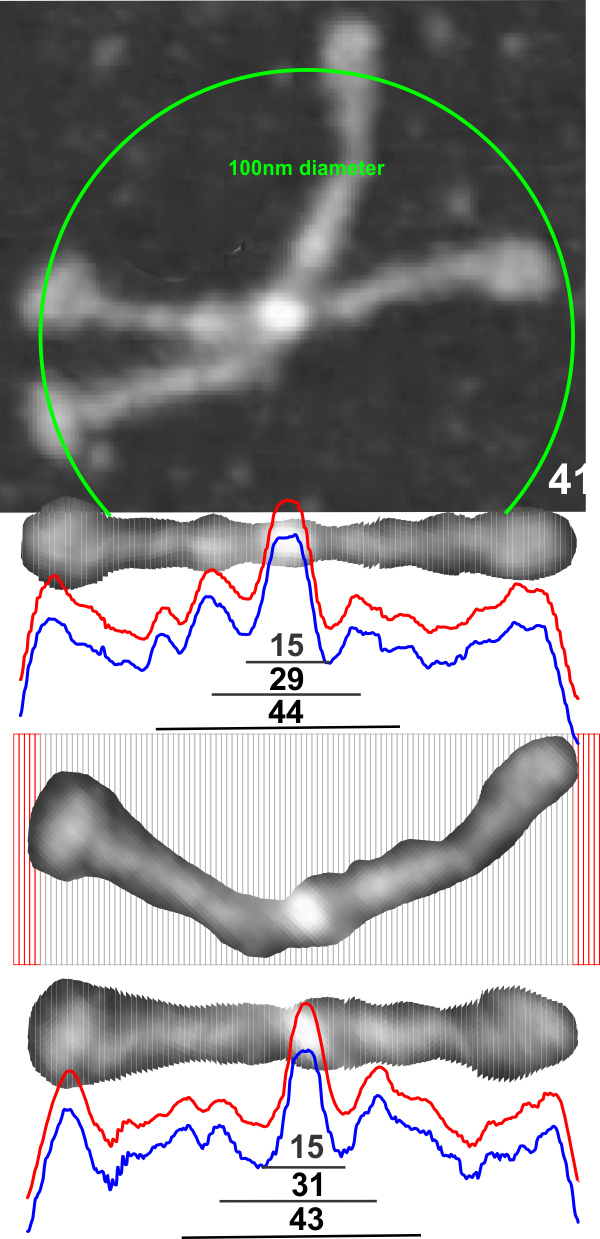 This is a simpler method for determining where the peaks and valleys are for the bright spots along the arms of the SP-D dodecamers (actually measuring both monomer arms end to end at the same time with the same N terminal juncture bright spots)
The cuts have been aligned with the 100nm marker for this particular AFM image and actually cut the image in 1nm slices. This is done using just before beginning of the greying of the two CRDs as the outer limits of the 100nm range (keeping in mind that the actual measurements made by many researchers is just ove 100nm for the width end to end of the dodecamer. They are just slightly over 100nm but I thought using 100nm as a standard (at the margin of the CRD would be an easy measurement to use as an enlargement constant (or control for the varied micron markers that researchers post that are clearly off the mark). It is my feeling that there are variations in prep of the SP-D dodecamers, but that basically the structures can be normalized to just over 100nm.
So when the sectioned areas of SP-D arms are cut into 100 slices, then the center of each of those slices centered horizontally will the other slices…. the light and dark areas are ligned up (as shown in previous posts) but NOW each slice represents 1nm. This makes it incredibly easy to measure the distances between peaks and valleys of the correspond look-up-tables, align them in the same dimension width-wise, and determine bright spots as well as how many nm they are separated from the CRD or N terminals. It just requires an aligning of the two plots under the image, and using the select tool to select however many 1nm segments occur (automatically counted as “objects”) within the selected area.
Busy with nothingness
I am reposting an interesting daily upbeat suggestions from one of the emails I get, this one from the Hour of Power. This line just grabbed me “Although it was hard work to not waste energy with busy nothingness”.
Wow, I felt this. This is the truth. I find that fast typing on the keyboard, or piano keys, moving objects around, creating new images, posts and figuring out new ways of analyzing this or that can occupy my mind 24/7/365, and while it is not physical exercise, it is hard work. There is good biological principle in the concept of a day of rest, and now, in 2020 (well not quite there yet) we don’t even dedicate one hour a week to purposeful “unplugging” from our world. Taking a day of rest is important, and the other 6 need to be physically exertive. This is a well proven method for staving off both mental and physical diseases.
There must be some hard wiring in humans that move us to do more, faster and I must have felt this anxiety previously (probalby daily haha) because I created this stained glass pattern to address my inability to “rest” “relax” “receive” “renew” “revive” many years ago. The title “be still and know that I am god”
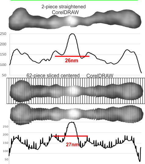
Happy with this analysis of grey scale density of SP-D images
After analyzing about 7 AFM images of SP-D dodecamers using the process of isolating the parallel arms, cutting into about 1.6 nm slices (that is around 62 slices per 100 nm SP-D molecule) and exporting to tiff (below is a comparison of the LUT from export as tiff vs export as jpg as analyzed in ImageJ) the plots are nice and they seem to represent quite accurately the number of “hand counted” bright peaks in each of the dimer-arms but clearly the export to jpg includes the “slices” which doesn’t happen with export to tiff.
I have not figure out yet how to blend the four arms into a single value per dodecamer, but that might actually not be necessary. At any rate, the next comparison will be with the shadowed SP-D dodecamers. It works really well on curved molecules… though It is required to expand the plots to a set 100nm this doesn’t change the number of peaks along each arm but will affect the distance measured for each bright spot (including the center).
Little surfactant protein D song and AA video
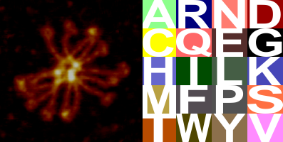 It is a little confusing to me why this melody haunts me, maybe there is an underlying predictability or drone that I can sense. I added the RCSB coloration and single letter designation for the amino acids. The colors are slightly representative of the relative acid and base tendencies of the amino acids. I am not sure what the colors represent in other than in those four AA where those properties are more pronounced like acid and base qualities. This is shown in the image on the right.
I would love to add a base or snare where the glycines occur… as those notes are relative low on the tone scale of the audio ( and it is a lot of work to go back and identify the glycines — of which there are many many.
Just an experiment, just a learning experience for me, no promises of absolute accuracy but pretty darn close.
Image on left is credited to other researchers (forgot whom) image on right is credited to the color coding of RCSB) assembly is credited to “moi”.
Reach Magazine – Cincinnati
First 25 pages devoted to pizza, second 3 to mexican food, next 3 to losing weight and fitness, last 5 for medical devices and lifts for those people who only read the first 28 pages.

Little surfactant protein D song: edit
I went back over the AA sequence and remade this audio and added the visual of the SP-D song. It didn’t change significantly, just some very obvious audio indications of where the collagen-like domain is. I find this so fun. You can see the drone of glycines while you listen to the audio in the image below, and it might be also present in the coiled coil of the neck… remember that the signal peptide accounts for the first 20 notes.
