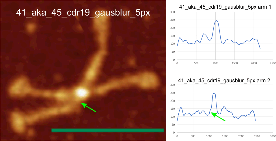
It is going to take a lot of convincing to persuade me that these four small peaks don’t exist: each I found in the trimers between the mostl unified peak of the N termini junction and the 4 glycosylation peaks on each of the trimers.  It stands to reason that they will not all 4, always show up, in all AFM images, but then little does show up in every image, so thats not going to be a sufficient rebuttal.

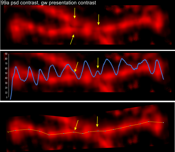
Here is an image from Arroyo et al, (which I call 99a).  While three obvious tiny peaks can be seen in this image that has been processed (not signal processed, but image processed), the 4th one is there as a tiny bump on the downslope of the presumed glycosylation peak.  Image on left shows tiny peaks pointed to by yellow in what i traced as “arm 1” and the green arrows show the tiny peaks in what I traced as “arm 2”.   The image processing filters applied to this image was contrast enhancement in photoshop and limit-range in gwyddion.  Relative peak heights in the plots to the right are skewed by the limit-range filter which eliminates all but a narrow range of brightness, but that does accentuate nicely the tiny peaks between the glycosylation peaks and the N termini junction (which on the plots lie above the arrows. Different dodecamers are seen for top-most image and the bottom 4 images.  Image proessing does not seem to alter where and when the tiny peaks by N are found.

For a long time I have wondered if there was any way i could determine whether the four trimers of an SP-D dodecamer could be attached not-end to end, but side to side. The images below show the first attempt to use image and signal processing to determine whether the N termini junction shows any indication of a side to side binding by showing differences in brightness within the broader scope of the N termini junction image as found with AFM.  These four plots (directions are crux 1 (shortest side to side of the N termini peak, that is, a line drawn from the widest angle of the dodecamer peak to the other wide angle); crus 2 (long direction of the peak (the narrow angle between the trimeric arms to the opposite side (also the narrow angle), as well as just the center N termini junction peak in each of the two hexamers (arm 1 and arm 2  (the latter two being two trimers each). With just this ONE dodecamer being analyzed so far, this is just a quick view…. but it seems that there are tiny peaks before the rising peak of the N termini in the arms, but not in the crux 1 and 2 measurements (see purple arrows on the images). It also seems that there is no flat place or depression in the plot of crux 1 (side to side from wide angle to wideangle), but there might be indication of a divot in the crux 2 and arm 1 and 2 plots.  This might indicate that the N termini junction has characteristics not normally described that might shed light on its structural nature.  Images below – top to bottom are, crux 1, crux 2, arm 1, arm 2, covering just what is plotted as the yellow line at the N termini junction.

The very pedestrian calculation of nm sq using a graphics program (which takes a few minutes) versus using Octave autofindpeaks.m is compared.  The values (except for a couple) are pretty close.  If i use the graphics program cut and pasting i can choose my own vertical lines for counting sq nm, but the data from octave are returned in a nice excel file. The problem is that If i disagree with the count and positions of the peaks then that is disconcerting (eg, the peak i colored green in the octave plot (peak 5) has a nm sq that looks totally out of line.  Why would it be 1105 while the peak beside it is only 922. So there is a calculation based on slope and stuff that i dont understand and would like not to use.

In addition, what i have not figured out how to do is to average in a baseline which is a predictable arch, going from CRDs on each end of the plot upwards just slightly to be at its highest under the N termini junction. I can delete grid from that part of the plot in the graphics program quite easily….. but have no clue how to do that in Octave.

I think i am going to step away from the peak area and just count peaks on either side of the N.  (which btw, i am predicting a small peak between the N termini junction and the glycosylation peak (in this case peaks 4 and 7 would be the latter,  peaks 5 and the peak to the right side of N termini junction that i chose to count.

The double peaks of the CRD are so clearly a result of different positions of the intividual trimer CRD, and so easily predictable as a tall peak before the tiny peak in the adjacent presumed (probably not neck) collagen-like domain that I would not give those individual numbers.  Octave wont separate them. Peaks 10 and 11 in Octave should be counted as a single peak.

Purpose: to find reliable ways to use image and signal processing together to suggest structural characteristics for proteins.

Small peaks in the grayscale plots of SP-D dodecamers include some that occur between the N term juncture and the glycosylation site.  They happen with regularity. I have not counted the number of times they show up the grayscale plots, but this dodecamer has three, and they are prominent, easily seen after image processing.  See arrows pointing to three small peaks. (likely a fourth exists, but did not show up here as a random artifact).  This dodecamer has been image processed (but not signal processed) and the molecule number is in the left corner of the top image, i.e. 99a.  The tiny peak shows up three times out of four, but is missing from the other hexamer where there is only one peak.  Just as an aside, the CRD (carbohydrate recognition domains) are nicely shown with this image processing protocol, sometimes all three CRD can be seen.  Also of note, the N terminus does not look like it has any valleys in the center.

I continue to thank Arroyo et al for the AFM images which I have processed the …. out of.

Here is a high contrast approach to image processing an AFM image of surfactant protein D (number 97 in this series). The processing is shown at the top of the image and it entailed altering contrast in both photoshop and gwyddion.  The plot actually is less informative than limiting the range (gwyddion) and applying the gaussian blur filter.  The increased contrast takes the N termini junction off the scale in brighness (255) and reduces the opportunity to compare peaks sizes (particularly with the adjacent glycosylation (alleged) peak which can vary. Comparison with previous posts on this blog shows different image processing, also concurrent signal processing and resulting LUT plots of the same SP-D molecule.

The advantage is however, a great visualization of the number of bright spots alone each of these arms of a dodecamer, clearly suggesting that there are regular structural elements. Per two previous posts… it looks like a hexamer (one line from carbohydrate recognition domain (the ends) to the other has a consistently visible more than 15 peaks.  Typically two peaks in the carbohydrate recognition domains, often two peaks in the glycosylation area (which might represent a level of glycosylation from 1, 2 to 3, one spot for each molecule of the trimer) and the stepwise peaks from the glycosylation site towards the neck region.

I dont really “like” this level of image processing (there has been no signal processing here), but it is informative.  It is easy to see peaks and compare them with underlying bright areas along the arms. Graphic made in CorelDRAW.

abbreviations: AFM – atomic force microscopy; LUT – look up tables (grayscale plots from ImageJ); gw – gwyddion software for AFM; photoshop – in this case, photoshop 6; CRD – carbohydrate domain;