Monthly Archives: August 2019

SP-D CRD to CRD measurements

Arroyo et al is perhaps the gold standard for measuring SP-D.  I keep coming back to this publication as the most apt to be correct in terms of measurements of surfactant protein D and while my intent was to go back and measure all the other images against each publications’ bar marker I am pretty convinced that the measurements from Arroyo et al are probably the best to use.

Comparing my analysis of a single dodecamer that appears in that publication and their analysis is interesting. I have used their micron marker as a scale bar for my analyses.

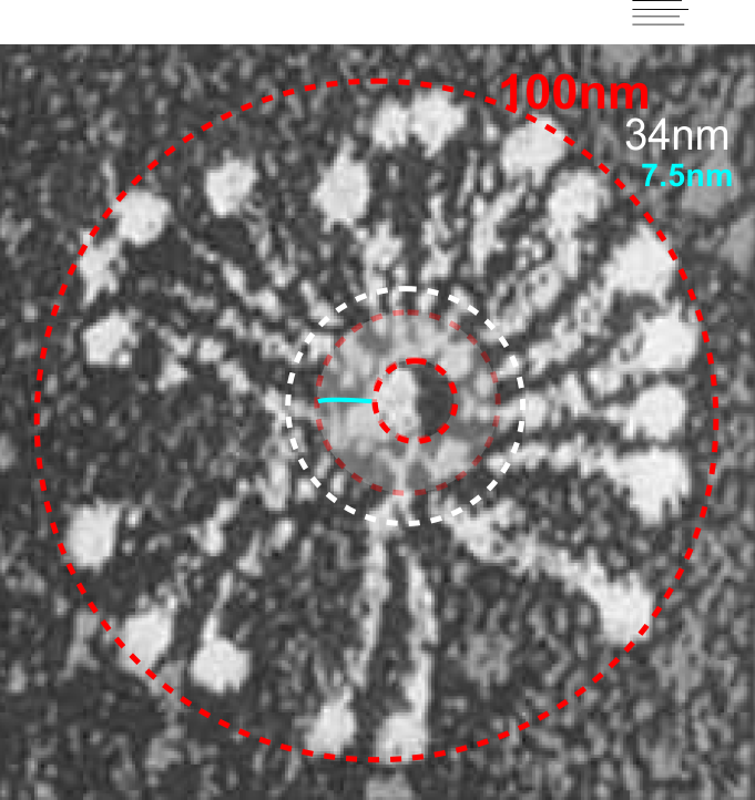
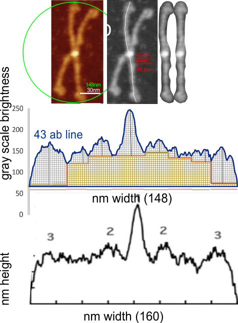
1) I have used a circle to estimate the size of the dodecamer (three out of four of the CRD are touching the circumference.  Arroyo calls peak 2, which is likely the peak that i call collagen-like domain peak 1 (because it is closest to the Nterminus) is variable in width but almost always less than the Ntermini peak of a dodecamer (as seen in Arroyo’s LUT (or height) plot and in almost all of the LUT plots that I have made as well. This peak is the brightest in shadowed images using TEM.

2) From peak 1 of the collagen-like domain the measurements (using 148 as the diameter of this molecule) is about 40nm and mean valley to valley of the two individual collagen 1 peaks in this particular molecule is about 20nm. The width of the peaks in Arroyo’s graph for CRD is about 28nm (using my 148nm diameter based on their 30nm bar marker).

3) Since this molecule is made up of identical monomers (12 of them) and since the Ntermini peak is NOT in the center of their plot (nor is it in the center of my LUT plots), I think that it is perfectly reasonable to “force” the half plots into equity. It is easy to see that the collagen 1 peak in the collagen like domain is wider on the side where the arm length is greater so i think that normalizing each side to “half” the distance would be a good (and fair) way to minimize the variability in size (which is most likely due to random falling onto the substrate during preparation (that is simplistic, yes).

4) the segmented line measurements are very close to the diameter measurements (case here where diameter of 148nm and segmented line measurements are 148.5 for the single arm measured is quite close. It is the same arm measured by Arroyo et al, who came up with a measurement of 160nm  which might be a little long.

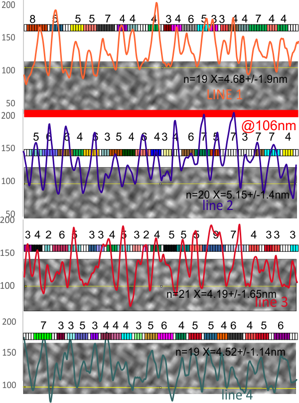
5) the third image (set of images) on the top row (left to right) show the same arm of the dodecamer cropped out, then sliced into 100nm (approx) segments, and those segments are aligned horizontally (technique described before on this blog) with the resulting image exported as tif for LUT tables using ImageJ. (that straightened arm is shown as the right-most image).

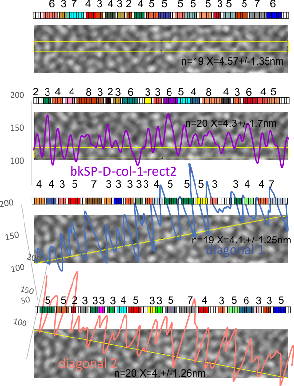
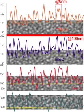
6) of all the dodecamers I have plotted, this happens to be what I called #43, labeled as such, and the two sets of arms are labeled a,b  and c,d  so that plots of each can be compared. I derived LUT tables from a) a single line (as per Arroyo) and as a rectangle in ImageJ.  There is some smoothing obtained by using a rectangle, but both methods produce pretty much the same results, just like the diameter vs the segmented line (measured twice, once in the vertical image, and once in the original analysis (red segmented lines at the base of the plot) to measure arm length are very close. The former is way easier however.

7) background was subtracted from the peak height (brightness or lightness, formerly lumanance) at the lowest point in the LUT tables within the molecule.

8) sq nm were determined for the  CRD. and the plot height and area as well.  All in all, i think there are some additional facts (namely two additional regularly occurring peaks in the collagen-like domains) and relative peak heights and areas as well as a simplified method for calculating the arm length of multimers of any kind (using both shadowed and AFM images, particularly relevant to those which form multimers like SP-A, SP-D, conglutinin C1Q etc.

9) comparing shadowed and AFM methods, and information derived from each (which is better? or more informative? only careful comparisons will tell. IT seems to me however that using the AFM for comfirmation, that the shadowed image show almost as much about the SP-D molecule as the AFM does. Maybe it is a little harder to ferret out.

I will say again, Arroyo did some nice morphometry…. for that i am appreciative. I dont think the resolution of their LUT plots (nm height but likely equivalent to the grayscale or LUT plots or relative sq nm in some measurements I have made) the are very conservative in choosing only one peak in the collagen-like domain…. I think consensus would say there are more.

Molecular models and micrographs: do they really equate

Atomic force microscopy images of fibrinogen, fibrin oligomers, and protofibrils and reconstruction of a protofibril model. (a-i). Images by high-resolution atomic force microscopy (used from a second hand image posted from original  of Drs. Anna D. Protopopova, Nikolay Barinov, Dmitry Klinov) from a post on Research Gate.

Sometimes putting the molecular model with the AFM image is a little difficult. Using the measure of 45 nm for the molecular model at the same magnification as the micrograph is marked (bar=30nm) something just looks out of proportion, however, the length of what would show up as between-peak brightness probably does equate to the model, but what is puzzling is the thickness of the two strands…  model vs micrograph where just a tiny portion of the micrograph (about the middle of the original (shown below) was cropped and enlarged to scale of the molecular model diagrams.


Shadowed rSP-D multimer with central dark area

This is the first shadowed image I have seen of rSP-D (original by oft cited Crouch et al) which has what I think is an Ntermini ring side by side configuration, leaving a dark hole in the center of the multimer. This has been seen with various AFM images which is where I first got the idea that the center might not be end to end Ntermini connections, but side to side.  Normalized to a diameter of 100nm (which is arbitrary since no ones measurements have been consistent) the central ring which might be the Ntermini is about 7nm in thickness, the white dotted circle is where the first and highest peak (in AFM images) would occur and is pretty clearly visible here at about 34nm diameter.  A comparison with the place for the 1st LUT peak in the AFM images would be necessary but it looks like it will coincide nicely. There is obvious disadvantage of background noise in shadowed images, but this particular image fits the concept that at least some of the time the Ntermini are side to side.

Relative to whole – SP-D

It seems because of the variations in reported size of SP-D dodecamers, and other multimers there is only one reasonable way to measure the different domains.  That is, as relative percents of the length of each of the hexameric arms (CRD-neck-collagen-like-Ntermini (together) collagen-like-neck-CRD.  Measuring from other people’s micrographs, and using two different electron microscopic techniques I have come up with measures from 100nm, 110, 130 and 135nm.  These differences can be due to a host of different methodologies, species, techniques. It seems expedient to adopt philosophy that measurements of different domains in SP-D are relative to 100% of the distance between the edges of CRD. That means that all future measures will be made using that distance as 100nm.  THis helps explain the slightly smaller measurements for the CRD used in estimating the LUT table peaks in the micrographs from different investigators whose techniques produce SP-D images of different diameters.

It is almost useless to have put “original magnification” as the magnification of an image in a manuscript, although I have been tempted and probably have done such, that is certainly the lazy way out and it gives absolutely no information as to the “real” magnification and enlargement of a micrograph.  case in point for crouch et al SP-D images coshadowed with collagen.

The dimensions and peak number in individual SP-D wont be adjusted….just the outer measurements of the whole.

I dont know why it didn’t strike me before but Crouch et al did not specify how they enhanced the dodecamers in their paper, clearly either they grey-brushed out the surrounding molecules, or they subjected the dodecamers they wanted to highlight to image processing. It makes a huge difference whether they enhanced the whole length of the dodecamers evenly or whether they used a contrast tool just sporadically over the micrograph to highlight the SP-D.  That is a huge deletion from the materials and methods.

Measuring shadow grains in TEM as diameters

Figuring out whether the shadow cast procedure for TEM obscures details in SP-D dodecamers (and other multimers) has been measured as LUT tables, and in yesterdays post it comes out to about 4.5nm. It occurred to me that easily measured grain size is to use a diameter of randomly selected grains. Picture below if one oft used in this analysis published by Crouch et al. The blue dots cover the CRD in SP-D, the salmon colored dots cover grains from the background. Using SP-D shadowed arms measured as hexamers (from one CRD to the other CRD — in a line (vector, with nodes, separated rotated to horizontal, then added together=135nm) then several arms taken for the mean, and normalized to 135nm, these grains are — relative to that number — almost identical to that measured using LUT tables.

It is n=94, 4.23nm diameter +/- 0.6nm (SD). The diameters would be smaller using this method (as observed) owing to the fact that there is a sharp line of demarcation in the circle overlying each grain, while in the LUT tables, the valleys are used (and there is a gradual extinction in the gray values around the edges of the grains in that type of measure thus increasing the width recorded).. the diameters are a quick and easy method, the LUT plots take time. Blue circles overlay CRD which measured in widest diameter come out to about 12.5nm in this micrograph (a dodecamer (two arms of the dodecamer measured) from this same micrograph but a different location showed using LUT plots a diameter of the CRD of about 13.5nm  — so this is close for a very small sample.


Wisdom from a comedian

Charlie Chaplin. It’s believed he wrote the poem below at age 70.

As I began to love myself
I found that anguish and emotional suffering
are only warning signs that I was living
against my own truth.
Today, I know, this is Authenticity.

As I began to love myself
I understood how much it can offend somebody
if I try to force my desires on this person,
even though I knew the time was not right
and the person was not ready for it,
and even though this person was me.
Today I call this Respect.

As I began to love myself
I stopped craving for a different life,
and I could see that everything
that surrounded me
was inviting me to grow.
Today I call this Maturity.

As I began to love myself
I understood that at any circumstance,
I am in the right place at the right time,
and everything happens at the exactly right moment.
So I could be calm.
Today I call this Self-Confidence.

As I began to love myself
I quit stealing my own time,
and I stopped designing huge projects
for the future.
Today, I only do what brings me joy and happiness,
things I love to do and that make my heart cheer,
and I do them in my own way
and in my own rhythm.
Today I call this Simplicity.

As I began to love myself
I freed myself of anything
that is no good for my health –
food, people, things, situations,
and everything that drew me down
and away from myself.
At first I called this attitude a healthy egoism.
Today I know it is Love of Oneself.

As I began to love myself
I quit trying to always be right,
and ever since
I was wrong less of the time.
Today I discovered that is Modesty.

As I began to love myself
I refused to go on living in the past
and worrying about the future.
Now, I only live for the moment,
where everything is happening.
Today I live each day,
day by day,
and I call it Fulfillment.

As I began to love myself
I recognized
that my mind can disturb me
and it can make me sick.
But as I connected it to my heart,
my mind became a valuable ally.
Today I call this connection Wisdom of the Heart.

We no longer need to fear arguments,
confrontations or any kind of problems
with ourselves or others.
Even stars collide,
and out of their crashing, new worlds are born.
Today I know: This is Life!

Sometimes I see things that make me laugh

Sometimes I see things that make me laugh – though more often than not, they make me cry, or feel disgusted.  But this made me laugh…. this morning driving to work at UC College of Medicine I spotted three new benches (in front of what was in ancient times “the college of medicine — aka the “old college of medicine”, then the “dean’s office” and now Kawolesky hall. These are a couple of metal benches. They are brand new and part of the renovation of the whole west part of the medical campus for the new public health building. NO TREES, and thus on a day like today which will be 90 degrees and no shade, I pity anyone going to “sit” on these benches…. one would certainly “braise (and/or braze) their glutei”.

Rotary shadowed background grains in this image are about 4.5nm

Confirming the background grain size in a particular image (so I can do LUT plots on a few SP-D dodecamers and type 1 collagen molecules for comparisoin with AFM images) is pretty uniform… varying about 1.5 nm  (n=79 x=4.63+/-1.45 nm.  This means that it might be possible to establish areas of greater luminance (brightness, lightness) on a 1-255 gray scale that correspond with different AA sequences in either (both) these molecules.

Individual lines and their nm thick peak-valleys, and a mean of all 4 lines together. Same plots as last week, same resource, just with the measurements of peak width (from lowest point in valley one side to the other.

and the two LUT plots made with rectangles, and two more plots made with diagonals. It seems that the rectangle might be the least good way to measure the nm of the shadowed background.  But all in all, it seems that a line, anyway you draw it will work just fine.

The next step is to see the width and variation in the type 1 collagen collagen and SP-D from the same micrograph.

Background grains in shadowed images of SP-D

Platinum shadowed images (with type 1 collagen) of SP-D (referenced so many times on this blog). A portion of one image with LUT plots as 4 lines (I also did 2 rectangles and 2 diagonals to see whether there was a directionality to the way the grains fell during shadowing). First little peak measured against the 135nm SP-D dodecamer (quickly judged by a diameter intersecting at least three of the four CRD) in the same micrograph shows the grains to be about 8 nm in width. I will measure each of these peaks and see whether there is too much variation to use such micrographs to determine peaks and valleys in actual dodecamers. Same image top to bottom, but the yellow line indicates where the LUT plots were made, they correspond well to the plots.